Synopsis

Keywords: Sparse & Low-Rank Models, Cardiovascular, Motion estimation; Motion correction; Low-Rank & Sparse;Time-resolved imaging

In this work we present a time-resolved (ungated, free-breathing) dynamic cardiac MRI method which disentangles and jointly estimates motion-fields and time-varying contrast images. Different sources of intensity variations are represented with L+S decompositions and motion-fields, that can naturally provide the information required for downstream tasks such as perfusion (contrast dynamics) and myocardial strain analysis (tissue dynamics). Results indicate the feasibility of disentangling the different sources of temporal intensity variations such as respiratory motion or contrast enhancement. Moreover, no breath holds nor ECG triggering/sorting are required since the time-resolved framework can simultaneously resolve the many overlapping dynamics from a continuous data-stream.

Introduction

Cardiac MRI (CMR) aims at non-invasive assessment of cardiovascular function. A typical examination analyses two types of cardiac dynamics: 1) perfusion (myocardial contrast uptake) and myocardial contraction (morphological).¹ A common approach in CMR re-sorts the data with respect to cardiac phase and reconstructs an average heart-beat.² However, for frequently occurring cardiac pathologies such as arrythmia, a complete time-resolved assessment of cardiac dynamics (contrast+morphological) could provide more valuable information and would remove the need for breath holds and ECG electrodes.^1,3

In this work, we propose a framework to jointly estimate time-resolved contrast and motion from ungated free-breathing acquisitions. For this purpose, we explicitly model motion-fields as well as exploit spatiotemporal intensity correlations in the time-varying MRI contrast. Our framework thereby automatically decomposes the spatio-temporal dynamics into several scales: larger scale tissue dynamics (e.g. breathing, myocardial contraction), and smaller scale contrast dynamics (e.g. perfusion).

Theory

We define target time-series images $$$\bf{I}=\left[{\bf{I}}_1,...,{\bf{I}}_\it{M}\right]$$$, reference contrast images $$$\bf{Q}=\left[{\bf{q}}_1,...,{\bf{q}}_\it{M}\right]$$$ and motion fields $$$\bf{D}=\left[{\bf{D}}_1,...,{\bf{D}}_\it{M}\right]$$$ for each dynamic $$$\it{t}$$$, up to $$$\it{M}$$$ total number of dynamics, and relate them as follows
$$\bf{I}_\it{t}\left(\bf{r}\right)=\bf{q}_\it{t}\left(\bf{D}_\it{t}^{\tt{-1}}\left(\bf{r}\right)\right)\cdot\det\left(\bf{\nabla}\bf{D}_\it{t}^{\tt{-1}}\right)\mathrm{,}\bf{}\tag{1}$$
where $$$\bf{r}=\it{}\left(x,y,z\right)$$$ are spatial coordinates and $$$\bf{\nabla}$$$ indicates the Jacobian. From equation 1, $$$\bf{I}_\it{t}$$$ is approximated by warping the reference image $$$\bf{q}_\it{t}$$$. This is a small but crucial extension to the MR-MOTUS framework⁴ where there is now a reference image for each $$$\it{t}$$$ giving the flexibility to use the low rank plus sparse (L+S) model⁵; thereby, the time-dependent image contrast variation is accounted for. In this work alternations are performed between 1) motion estimation for determining the motion fields $$$\bf{D}$$$ and 2) motion correction for determining the time-dependent contrast changes $$$\bf{Q}$$$. We briefly describe both reconstruction steps.
1) Motion Estimation
The following model $$$\bf{F}$$$ is an extension of the MR-MOTUS model⁶ which explicitly relates the reference contrast images $$$\bf{Q}$$$ to the motion fields $$$\bf{D}$$$ for the measured k-space data $$$\bf{s}_\it{t}$$$
$$
\bf{s}_\it{t}\left(\bf{k}\right)=\bf{F}\left(\bf{D}_\it{t}|\bf{q}_\it{t}\right)=\int_{\Omega}\bf{q}_\it{t}\left(\bf{r}\right)e^{-i2\pi\bf{k}\cdot\bf{D}_\it{t}\left(\bf{r}\right)} d\bf{r}\mathrm{,}\bf{}\tag{2}
$$
where $$$\bf{k}=\it{}\left(k_x,k_y,k_z \right)$$$ are k-space coordinates. To estimate motion, the following minimization problem is solved given the current motion-corrected estimation of $$$\bf{Q}$$$ from step 2
$$
\left[\bf{\Phi}^\it{*},\bf{\Psi}^\it{*}\right]=\underset{\bf{\Phi}\bf{\Psi}^\it{T}=\left[\bf{D}_\tt{1},...,\bf{D}_\it{M}\right]}{\mathrm{argmin}}\sum_t^M||\bf{F}\left(\bf{D}_\it{t}|\bf{q}_\it{t}\right)-\bf{s}_\it{t}||_\tt{2}^2+\lambda_{\text{TV}}\mathrm{TV}\left(\bf{D}\right)+\lambda_\text{T}\it{}||\bar{\bf{D}}\it{}||_\tt{2}\mathrm{.}\bf{}\tag{3}
$$
Here, $$$\bf{\Phi}$$$ and $$$\bf{\Psi}$$$ represent the spatial and temporal low rank approximation for motion fields, respectively. In addition to the total variation ($$$\text{TV}$$$) spatial regularization of the motion fields, a penalty on the temporal mean $$$\bar{\bf{D}}$$$ is added. $$$\lambda_{\tt{TV}}\mathrm{>0}$$$ and $$$\lambda_\text{T}\mathrm{>0}$$$ denote the regularization parameters. Equation 3 is a non-linear problem which is solved with L-BFGS.
2) Motion Correction
Given the current motion estimation of $$$\bf{D}_\it{t}$$$ from step 1, the following minimization problem is solved
$$
\left[\bf{L}^\it{*},\bf{S}^\it{*}\right]=\underset{\bf{Q}=\left[\bf{L}+\bf{S}\right]}{\mathrm{argmin}}\sum_t^M||\bf{F}\left(\bf{q}_\it{t}|\bf{D}_\it{t}\right)-\bf{s}_\it{t}||_\tt{2}^2+\lambda_{\tt{L}}\it{||}\bf{L}\it{||}_*+\lambda_\tt{S}\it{}||\mathcal{F}\bf{S}\it{}||_\tt{1}\mathrm{.}\bf{}\tag{4}
$$
Here, the reference images $$$\bf{Q}$$$ are decomposed into low-rank $$$\bf{L}$$$ and sparse $$$\bf{S}$$$ components $$$\bf{Q}=\bf{L}+\bf{S}$$$ like in [5], and $$$\mathcal{F}$$$ is a temporal Fourier transform. The regularization terms forces the reference images to be in the same motion state, with a slight flexibility to describe signal variations such as dynamic contrast enhancement. $$$\lambda_\tt{L} \mathrm{>0}$$$ and $$$\lambda_\tt{S}\mathrm{>0}$$$ denote the regularization parameters. Equation 3 is a linear problem which can be solved with standard L1 optimization routines.⁷
Alternating Scheme
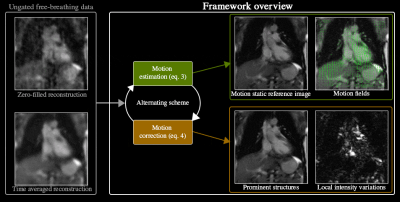
Equations 3 and 4 are solved in an alternating scheme. This allows to estimate motion-fields from highly under sampled data (Eq. 3), then subsequently use that estimation to reconstruct a motion corrected image (Eq. 4). Repeating this scheme with suitable parameters results in different motion dynamics $$$\bf{D}$$$, $$$\bf{L}$$$ and $$$\bf{S}$$$, as well as reconstruct motion-corrected reference contrast images $$$\bf{Q}$$$. An overview of the pipeline is presented in Figure 1.

Methods

Two datasets of 2D cine CMR (one with contrast enhancement) were used. K-space was retrospectively simulated for this data. The dataset with contrast enhancement was used to test whether the different dynamics could be separated correctly by the framework. The alternating reconstruction scheme was initialized with $$$\bf{D} = \bf{0}$$$ for both datasets.
Total reconstruction time for one alternating iteration (Equation 3 and Equation 4) was around 5 minutes for 2D data on a PC with 64 threads.

Results

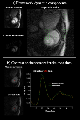
Figure 1 shows an overview of the framework.

Figure 2 shows tests whether the framework could separate the signal modulation by contrast-agent uptake with the $$$\bf{S}$$$ component and (b) the breathing motion could be described by the motion-fields $$$\bf{D}$$$.

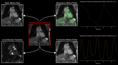
Figure 3 shows tests whether the framework could correctly separate (i) local intensity variations, (ii) respiratory motion and (iii) myocardial contraction.

Discussion

In this work we presented a time-resolved (ungated and free-breathing) dynamic CMRI method which disentangles and jointly estimates motion field and time-varying contrast images. Different sources of intensity variations were represented with L+S decompositions and motion-fields, that could naturally provide the information required for downstream tasks such as perfusion (contrast dynamics) and myocardial strain analysis (tissue dynamics). Results indicate the feasibility of disentangling the different sources of temporal intensity variations such as respiratory motion or contrast enhancement. Moreover, no breath holds nor ECG triggering/sorting are required since the time-resolved framework can simultaneously resolve the many overlapping dynamics from a continuous data-stream. Overall, this method presents new possibilities of time-resolved and free-breathing assessment of cardio-vascular imaging.

In conclusion, we present a new approach for time-resolved CMRI using a multi-scale dynamics decomposition. The simulations from this study warrant further investigation on 3D and prospectively acquired in-vivo data.

Acknowledgements

This research is funded by the Netherlands Organisation for Scientific Research (NWO), domain Applied and Engineering Sciences, Grant number 19003.