0840
Deconvolution for Hyperpolarized Magnetic Resonance Imaging
Jack J. Miller1,2, Nikolaj Bøgh1, Andrew Tyler3, Justin Y C Lau4, Esben Søvsø Szocska Hansen1, Michael Væggemose1,5, Oliver Rider6, Damian Tyler6, and Christoffer Laustsen1
1The MR Research Centre, Aarhus University, Aarhus, Denmark, 2OCMR, Radcliffe Department of Medicine, University of Oxford, Oxford, United Kingdom, 3King's College London, London, United Kingdom, 4GE Healthcare, Schenectady, NY, United States, 5GE Healthcare, Brøndby, Denmark, 6OCMR, RDM, University of Oxford, Oxford, United Kingdom
1The MR Research Centre, Aarhus University, Aarhus, Denmark, 2OCMR, Radcliffe Department of Medicine, University of Oxford, Oxford, United Kingdom, 3King's College London, London, United Kingdom, 4GE Healthcare, Schenectady, NY, United States, 5GE Healthcare, Brøndby, Denmark, 6OCMR, RDM, University of Oxford, Oxford, United Kingdom
Synopsis
Keywords: Hyperpolarized MR (Non-Gas), Data Analysis
Hyperpolarized metabolic imaging is translating into clinical practice. However, the desire to obtain chemical, spatial and temporal information combined with the finite and non-renewable exogenous magnetisation provided by hyperpolarized techniques often results in imaging sequences with a poor point-spread function. Here we compare multiple deconvolution algorithms to improve apparent reconstructed resolution, as is commonly performed in PET imaging. We show that deconvolution can significantly improve the reconstructed resolution of hyperpolarized images.Introduction
Hyperpolarized imaging sequences aim to image the metabolic conversion of substrates across space and time. As the finite and non-renewable exogenous magnetisation generated by the technique is depleted by each RF pulse played, and the time available for imaging is limited, most approaches widely used feature a rapid imaging readout, either with a direct spectral readout,[1,2] spectra-spatial selective excitation[3,4] or IDEAL-like decomposition for chemical shift encoding.[5,6] Additionally, compressed sensing approaches or other undersampled readout techniques (such as the use of a hybrid spiral trajectory[7]) have been taken to further accelerate the imaging readout.[8–10]All of these approaches yield image datasets with a comparatively poor point-spread function (PSF). In some cases these PSFs can be significantly larger than the nominal voxel size present within each image.[11–13] This effectively degrades the resolution of the “true” underlying image by convolution with the PSF. Additionally, after reconstruction, image-domain noise may not be normally distributed about zero, either because (a) the image-domain SNR is low and noise is Rician; (b) because the typically spatially regularised image-domain reconstruction algorithms employed do not guarantee that the image-domain SNR is white; or (c) a combination of the above.
We therefore investigated the efficacy of several deconvolution algorithms on the reconstruction of hyperpolarized imaging datasets. We note that most algorithms assume either Gaussian or Poissonian noise statistics, and either require perfect knowledge of the PSF, an estimate of the PSF (“myopic deconvolution”) or no knowledge of the PSF beyond an initial estimate (“blind”).
Methods
To highlight the role played by the PSF in rapid imaging sequences, we computed the PSF for two previously published spiral trajectories, a “conventional” Hargreaves imaging readout, and a previously-proposed multiresolution hybrid-shot spiral sampling trajectory.[7] These PSFs are shown in Figure 1. A computational brain phantom was discretised and “imaged” through a coarse spiral trajectory in order to provide a series of images of varying SNR (degraded through the mechanism of T2* decay) as described previously.[7]We compared several different deconvolution algorithms that have previously been widely used either in the context of nuclear medicine or optical imaging. Briefly, these were, the Wiener filter with a known PSF, as implemented either by Sci-Kit image with (1) a manual estimate of the image-domain Gaussian noise intensity[14]; (2) an automatic estimate of image-domain noise;[15] (3) MATLAB’s implementation of a regularised Wiener filter;[16] (4) Lucy-Richardson deconvolution as implemented in Sci-Kit image[17,18]; (5) a modified form of the AIDA “myopic” deconvolution algorithm, modified to have an appropriate form of the expected noise distribution from magnitude-mode MR images; (6) a standard MATLAB implementation of a maximum-likelihood blind deconvolution algorithm[19] or (7) regridding with a higher nominal voxel size provided by using a finer grid for a resulting NUFFT. We subsequently computed both mean squared image-domain error, and image self-similarity compared to the analytically known “ground truth”. We validated these experiments by undertaking a proton comparison between low-resolution gradient echo images obtained with a poor PSF and higher-resolution proton images. Finally, we performed a retrospective reconstruction of previously acquired human hyperpolarized data, obtained from the kidneys (constant spiral) or heart (hybrid spiral).
Results
As shown in Figure 2, different implementations of nominally similar algorithms performed quantitatively distinctly at differing SNR levels. We observed that, in the limiting SNR environment often encountered in time-resolved hyperpolarised imaging, regularised deconvolution algorithms were able to reconstruct meaningful images that outperformed regridding. We noted that the ideal algorithm appeared to be a function of SNR. We noted that the modified (myopic) AIDA algorithm was approximately the most performant over the low-but-usable SNR region expected to be encountered in metabolite images.We obtained a substantial improvement in the appearance of Gibbs ringing in a proton resolution phantom (Figure 3) when aiming to restore blurring caused by the finite PSF of the acquisition. As expected, quantitative image metrics obtained from downsampled and signal-volume corrected higher resolution images were significantly improved across all slices by the use of the modified AIDA algorithm (p < 0.05 via Wilcox test).
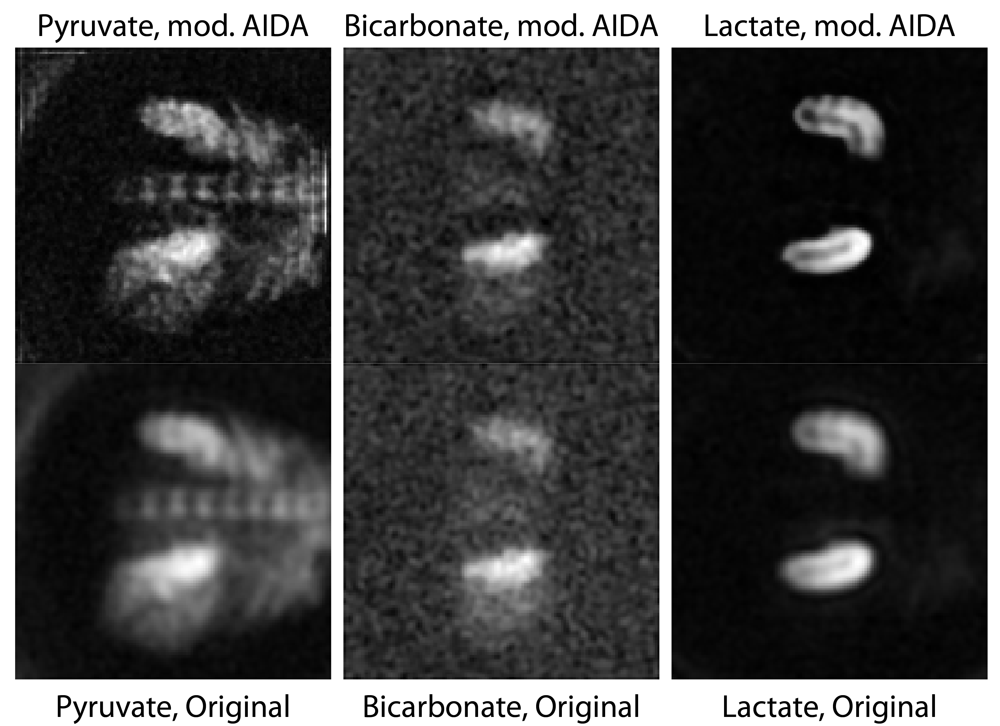
In the kidneys, we observed enhanced distinction between the renal cortex and medulla (lactate image) and the presence of a slight edge-of-acquisition artefact (pyruvate image) post deconvolution, with clearer delineation of the spinal vasculature (Figure 4). Cardiac images previously obtained with a hybrid spiral trajectory in a patient post myocardial infarction[20] showed enhanced myocardial contours (bicarbonate image) and greater splenic definition (lactate image; Figure 5).
Discussion and Conclusion
Deconvolution algorithms are widely used in other areas of imaging science, such as nuclear medicine and astronomy, and are accepted as ameliorating deleterious PSFs. However, deconvolution is an ill-posed inverse problem and prone to noise amplification. The methods explored all filter signals consistent with noise of known statistics and AIDA additionally contains an image-domain clique potential regularisation term that aids the reconstruction of natural looking images.Given the fundamental physical limitations on hyperpolarised imaging acquisitions, it is often the case that datasets are obtained in a low SNR regime and with a poor PSF. We have demonstrated that the use of an appropriate algorithm may be able to avoid the problem of Gibbs ringing, and shown physiologically- plausible improvements in image quality in the heart and kidneys.
Acknowledgements
We would like to acknowledge support from the Novo Nordisk Foundation (NNF21OC0068683); the British Heart Foundation (refs.~RG/11/9/28921, RE/13/1/30181, FS/19/18/34252 and FS/14/17/30634); the Engineering and Physical Sciences Research Council (EPSRC) and Medical Research Council (MRC) (EP/L016052/1); and the Colleges of St.~Hugh's and Somerville in the University of Oxford. We would furthermore like to acknowledge the University of Oxford British Heart Foundation Centre for Research Excellence (RE/13/1/30181), and the NHS National Institute for Health Research Oxford Biomedical Research Centre program.References
[1] R. Schmidt, C. Laustsen, J.-N. N. Dumez, M. I. Kettunen, E. M. Serrao, I. Marco-Rius, K. M. Brindle, J. H. Ardenkjaer-Larsen, L. Frydman, Journal of Magnetic Resonance 2014, 240, 8–15.[2] M. S. Ramirez, J. Lee, C. M. Walker, V. C. Sandulache, F. Hennel, S. Y. Lai, J. A. Bankson, Magnetic resonance in medicine 2014, 72, 986–95.[3] A. Z. Lau, A. P. Chen, R. E. Hurd, C. H. Cunningham, NMR in biomedicine 2011, 24, 988–96.[4] J. J. Miller, A. Z. Lau, I. Teh, J. E. Schneider, P. Kinchesh, S. SmarT, V. Ball, N. R. Sibson, D. J. Tyler,Magnetic Resonance in Medicine 2016, 75, 1515–1524.[5] M. Durst, U. Koellisch, A. Frank, G. Rancan, C. V. Gringeri, V. Karas, F. Wiesinger, M. I. Menzel, M.Schwaiger, A. Haase, R. F. Schulte, NMR in Biomedicine 2015, 28, 715–725.[6] F. Wiesinger, E. Weidl, M. I. Menzel, M. A. Janich, O. Khegai, S. J. Glaser, A. Haase, M. Schwaiger, R. F. Schulte, Magnetic resonance in medicine : official journal of the Society of Magnetic Resonancein Medicine / Society of Magnetic Resonance in Medicine 2012, 68, 8–16.[7] A. Tyler, J. Lau, V. Ball, K. Timm, T. Zhou, D. Tyler, J. Miller, Magnetic resonance in medicine 2021,85, 790–801.[8] M. H. Deppe, J. M. Wild, J. Parra-Robles, K. J. Lee, S. Ajraoui, S. R. Parnell, Magnetic Resonance inMedicine 2010, 63, 1059–1069.[9] B. J. Geraghty, J. Y. C. Lau, A. P. Chen, C. H. Cunningham, Magnetic Resonance in Medicine 2017,77, 538–546.[10] S. Hu, M. Lustig, A. P. Chen, J. Crane, A. Kerr, D. A. C. C. Kelley, R. Hurd, J. Kurhanewicz, S. J.Nelson, J. M. Pauly, D. B. Vigneron, J. Magn. Reson. 2008, 192, 258–264.[11] D. Chaimow, A. Shmuel, A More Accurate Account of the Effect of K-Space Sampling and SignalDecay on the Effective Spatial Resolution in Functional MRI, 2017.[12] M. Schär, B. Strasser, U. Dydak, eMagRes 2016, DOI 10.1002/9780470034590.emrstm1454.[13] J. J. Miller, J. T. Grist, S. Serres, J. R. Larkin, A. Z. Lau, K. Ray, K. R. Fisher, E. Hansen, R. S.Tougaard, P. M. Nielsen, J. Lindhardt, C. Laustsen, F. A. Gallagher, D. J. Tyler, N. Sibson, ScientificReports 2018, 8, 15082.[14] J. Immerkær, Computer Vision and Image Understanding 1996, 64, 300–302.[15] F. Orieux, J.-F. Giovannelli, T. Rodet, JOSA A 2010, 27, 1593–1607.[16] R. C. Gonzalez, R. C. Woods, R. E. Woods, Digital Image Processing, Addison-Wesley, 1992.[17] L. B. Lucy, The Astronomical Journal 1974, 79, 745.[18] W. H. Richardson, JOSA 1972, 62, 55–59.[19] T. J. Holmes, S. Bhattacharyya, J. A. Cooper, D. Hanzel, V. Krishnamurthi, W.-c. Lin, B. Roysam, D. H.Szarowski, J. N. Turner in Handbook of Biological Confocal Microscopy, (Ed.: J. B. Pawley), SpringerUS, Boston, MA, 1995, pp. 389–402.[20] A. Apps, J. Y. C. Lau, J. J. J. J. Miller, A. Tyler, L. A. J. Young, A. J. M. Lewis, G. Barnes, C. Trumper,S. Neubauer, O. J. Rider, D. J. Tyler, JACC: Cardiovascular Imaging 2021, 0, DOI 10.1016/j.jcmg. 2020.12.023.Figures
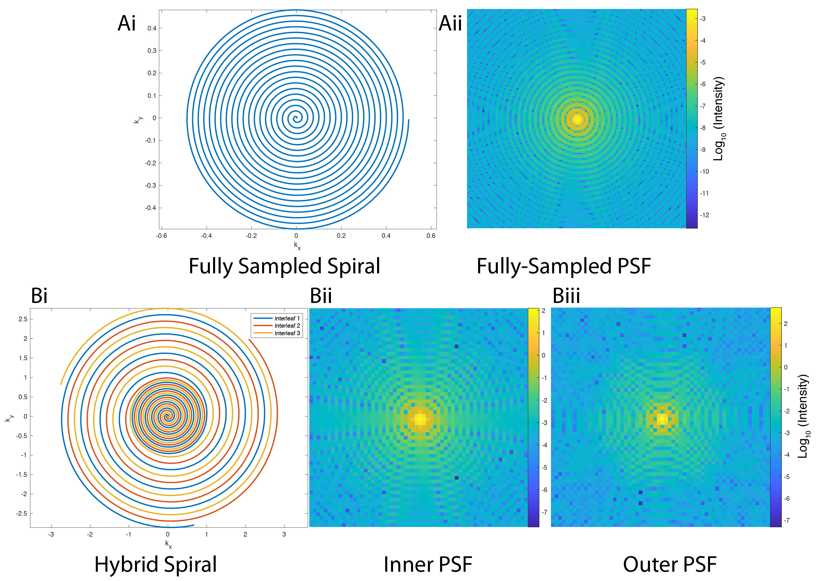
The two spiral k-space trajectories considered in this work and their associated point-spread functions. A "conventional" Hargreaves spiral and associated PSF is shown in Ai/ii. In comparison, Bi: A hybrid-shot spiral (HSS) k-space trajectory with both the PSF of (Bii) the inner, fully-sampled region shown from a single-shot spiral and (Biii) the outer, full PSF reconstructed from three-interleaves. All PSFs are shown on a logarithmic scale.
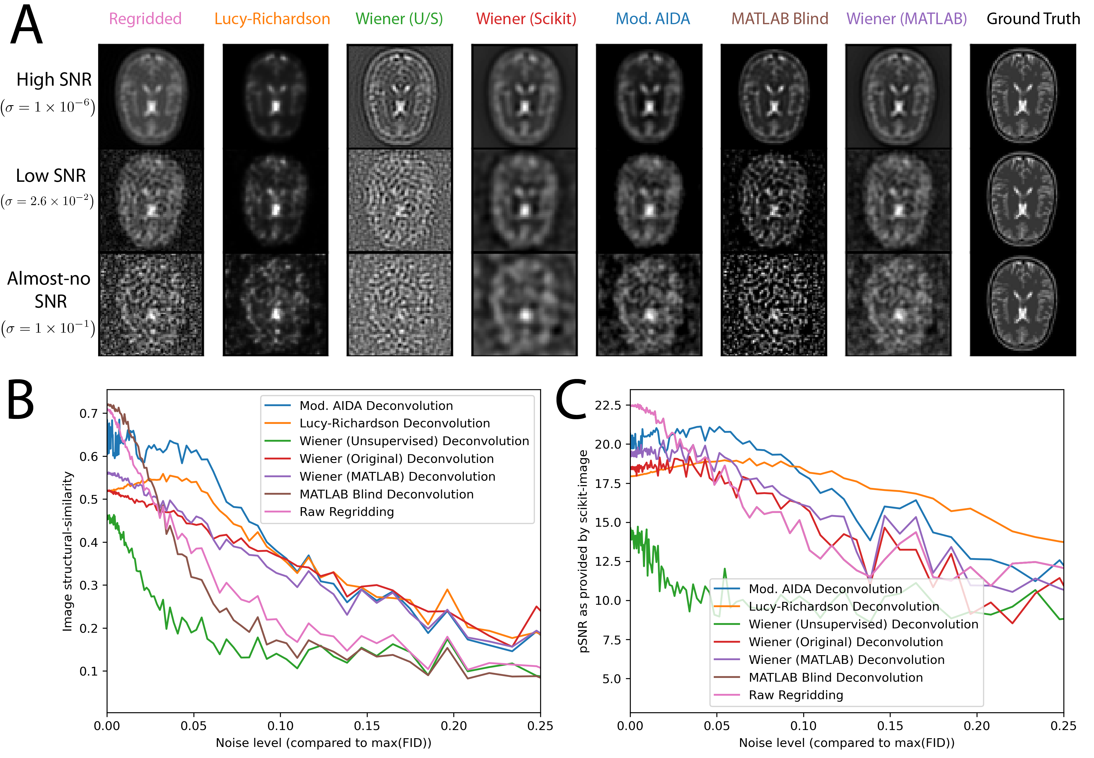
A: Representative post-deconvolution images of a computational brain phantom, obtained via the algorithms tried. Data are shown at three different SNR-levels, where $$$\sigma$$$ refers to the the standard deviation of the noise added to the FID in comparison to the initial maximum signal. B, C: The resulting quantified image structural similarity and normalised pSNR show that deconvolution approaches can quantitatively improve the reconstruction of low resolution datasets.
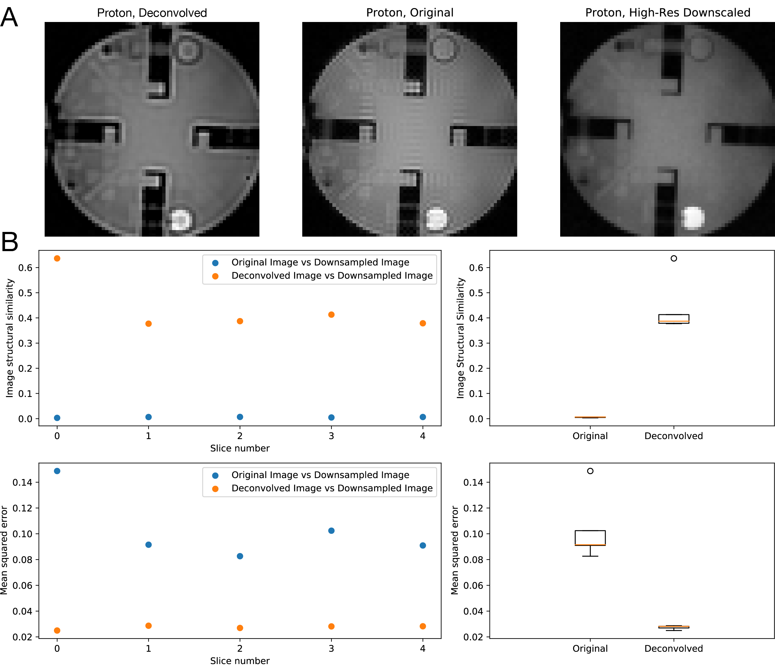
The (modified) AIDA algorithm applied to a proton resolution phantom with an analytic estimate of the point spread function significantly reduces visible Gibbs ringing compared to a downsampled high-resolution image (A). This improved both the image structural similarity score (which increased across all five slices of the phantom scanned) and mean-squared error (which likewise decreased) (B).
Reconstructed pyruvate, bicarbonate and lactate images from human kidneys obtained with the use of a spectral-spatial excitation and the Hargreaves spiral trajectory. The modified AIDA method was used for image-domain deconvolution. Of note are the reconstruction of the distinction between the renal cortex and medulla in the lactate image, and the presence of a slight edge-of-acquisition artefact arising in the pyruvate image post deconvolution, together with better delineation of the spinal vasculature.
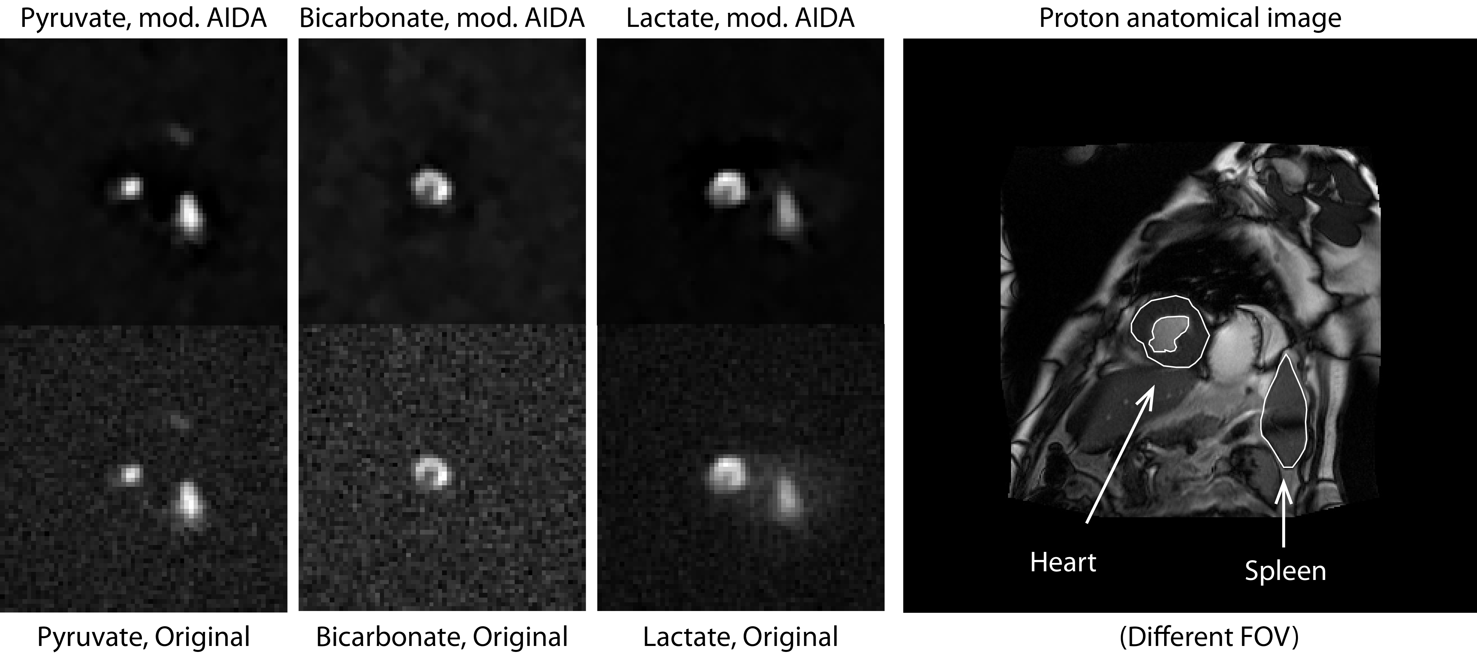
Reconstructed pyruvate, bicarbonate and lactate images from the human thorax obtained with the use of spectral-spatial excitation and the modified Hybrid shot sequence (HSS) shown previously, reconstructed using the three-interleaved data at full resolution and deconvolved with mod. AIDA. This patient was acute post MI and a clear reduction in bicarbonate is visible in the infarcted segment of the myocardium. What deconvolution makes more apparent however is the localisation of pyruvate perfusion and lactate production to the spleen, without the generation of spurious signal.
DOI: https://doi.org/10.58530/2023/0840