Synopsis

Keywords: Parallel Imaging, Image Reconstruction, Quantitative Imaging, White Matter

Recently, acceleration of 3D multi-echo gradient-echo (mGRE) acquisition for myelin water imaging (MWI) has been achieved using parallel imaging (PI) or deep learning network. However, these methods typically allow a low acceleration factor (R) for MWI because of the high sensitivity of the MWI estimation routine with respect noise/artifacts. Here, we developed a reconstruction deep learning network called the jointly unrolled cross-domain optimization-based spatio-temporal reconstruction network. According to retrospective and prospective reconstruction results, the proposed method achieved high-fidelity performance on the reconstructed mGRE images and MWI maps.

INTRODUCTION

Multi-echo gradient-echo (mGRE)-based myelin water imaging (MWI) can generate an indirect map of the myelin sheath in the brain ^1,2. Accelerating the acquisition of MWI is a challenging task due to the residual artifacts on the reconstructed mGRE images. Previous studies for accelerated 3D mGRE acquisition have been developed using parallel imaging (PI) and neural networks ^3,4. On the other hand, these methods typically allow a low acceleration factor (R) of up to 2 for mGRE acquisition because of the high sensitivity to noise/artifacts. Specifically, the residual artifacts of early echo images have a serious effect on the MWI estimation ^5,6.
In this study, to overcome these limitations, we developed a jointly unrolled cross-domain optimization-based spatio-temporal reconstruction network that can accelerate 3D whole brain mGRE acquisition for MWI with a resolution of 1.5mm×1.5mm×1.5mm. The network could correct local and global artifacts by iterating between the image and k-space domains. The proposed method achieved high-fidelity reconstruction performance and accelerated the acquisition time to only 2:22 minutes (approximately 6.5-fold acceleration).

METHODS

[Data acquisition]
All in-vivo data were acquired on a clinical 3T MRI scanner (Magnetom Tim Trio; Siemens Medical Solution, Erlangen, Germany). 3D mGRE scan protocol for fully-sampled acquisition: field of view (FOV)=240mm×240mm×144mm, resolution=1.5mm×1.5mm×1.5mm, 52 coils, TR=60ms, number of echoes=15 (TE₁=1.71ms, TE₁₅=30.83ms, ΔTE=2.21ms), flip angle=20˚, and total scan time=15:23 minutes. Moreover, we acquired and reconstructed prospective accelerated data by modifying GRE sequence (2:22 minutes).
[Reconstruction algorithm]
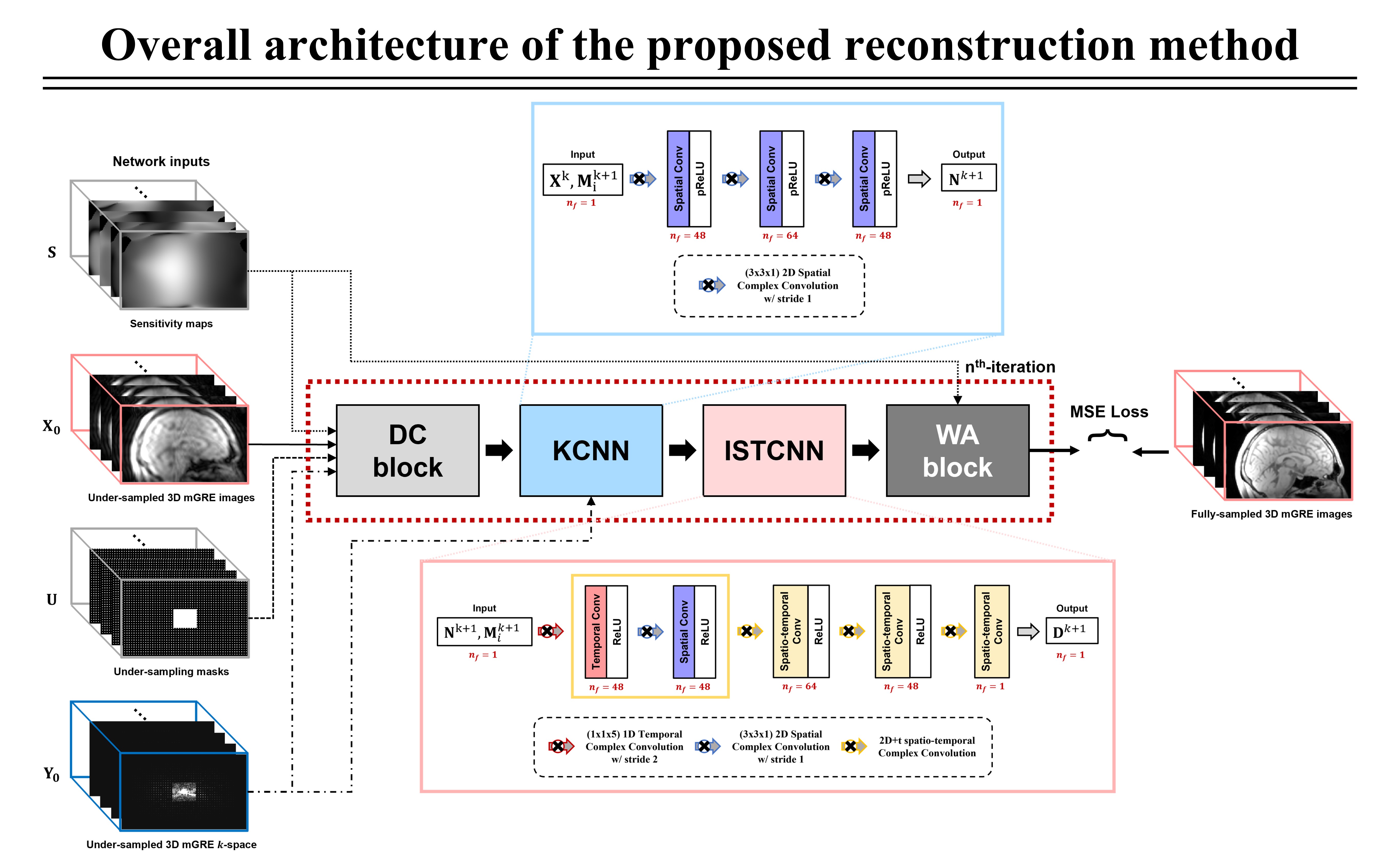
The network architecture is shown in Fig.1. The proposed network takes four inputs: under-sampled k-space data, coil sensitivity maps, under-sampling mask, and coil-combined under-sampled mGRE images. For the training data, a retrospective under-sampling process of the fully-sampled data in the first (R₁) and second (R₂) phase encoding line directions (R=R₁×R₂) was performed. The center portion of the k-space, named auto-calibrating signal (ACS), was sampled for coil compression ⁷ (8 compressed coils) and calibration of sensitivity map usages (30 × 24) from ESPIRiT ⁸ technique.
The proposed network consists of four main blocks:
DC block (data consistency block)
$$m_i^{k+1}=arg\min_{m_{i}}\frac{λ}{2}\sum_{i=1}^{n_c}\left\Vert UF(m_i)-y_i \right\Vert_2^2+\frac{α}{2}\sum_{i=1}^{n_c}\left\Vert m_i-S_ix^k\right\Vert_2^2\ \ \ (1)$$
KCNN block (k-space denoiser block)
$$n^{k+1}=arg\min_{n}\frac{β}{2}\left\Vert n-F\left(\sum_{i=1}^{n_c}S_i^Hm_i^{k+1}\right)\right\Vert_2^2\ \ \ (2)$$
ISTCNN block (image space denoiser block)
$$d^{k+1}=arg\min_d\frac{β}{2}\left\Vert d-F^{-1}(n^{k+1})\right\Vert_2^2\ \ \ (3)$$
WA block (weight averaging block)
$$x^{k+1}=arg\min_{x}\frac{α}{2}\sum_{i=1}^{n_c}\left\Vert m_i^{k+1}-S_ix \right\Vert_2^2+\frac{β}{2}\left\Vert d^{k+1}-x\right\Vert_2^2\ \ \ (4)$$ $$s.t. d=x, n=F(x), m_i=S_ix, i\in\left\{1, 2, ..., n_c\right\}, k\in\left\{1, 2, ..., n_{it}\right\}$$
where x denotes complex-valued MR image, y_i denotes under-sampled k-space data measured from the i^th MR receiver coil, S_i is i^th coil sensitivity map, F denotes Fourier transform (FT) operator, and U denotes under-sampling mask. By applying the variable splitting technique ⁹ with regularization, the first constraint d = x, n = F(x) decomposes x in the regularization term so that it explicitly formulates a denoising problem. The second constraint m_i = S_ix allows the decomposition of S_ix from UF(S_ix) in the data consistency term to alleviate matrix calculation.
Each layer sequentially incorporates frequency (5) and image (6) space convolutions:
$$n^{k+1}=σ\left\{w^k*F\left(\sum_{i=1}^{n_c}S_i^Hm_i^{k+1}\right)\right\}+F\left(x^k\right)\ \ \ \ \ \ s.t. σ(x)=x+ReLU\left(\frac{x-1}{2}\right)+ReLU\left(-\frac{x+1}{2}\right)\ \ \ (5)$$
$$d^{k+1}=σ'\left\{w'^k*WA\left(F^{-1}(n^{k+1}),\sum_{i=1}^{n_c}S_i^Hm_i^{k+1}\right)+b\right\}+\sum_{i=1}^{n_c}S_i^Hm_i^{k+1}\ \ \ (6)$$
where w and w' denote weight matrices of the frequency and image domains respectively, σ denotes alternative nonlinear activation function ¹⁰, σ' denotes rectified linear unit (ReLU) activation function, b denotes bias of the image domain, and WA denotes weight averaging operator. The spatio-temporal convolutions were implemented in the ISTCNN block as a 2D+t convolution to efficiently compensate for T2* temporal information. Finally, artificial neural network (ANN)-based MWI reconstruction method was applied for MWI estimations ¹¹.

RESULTS

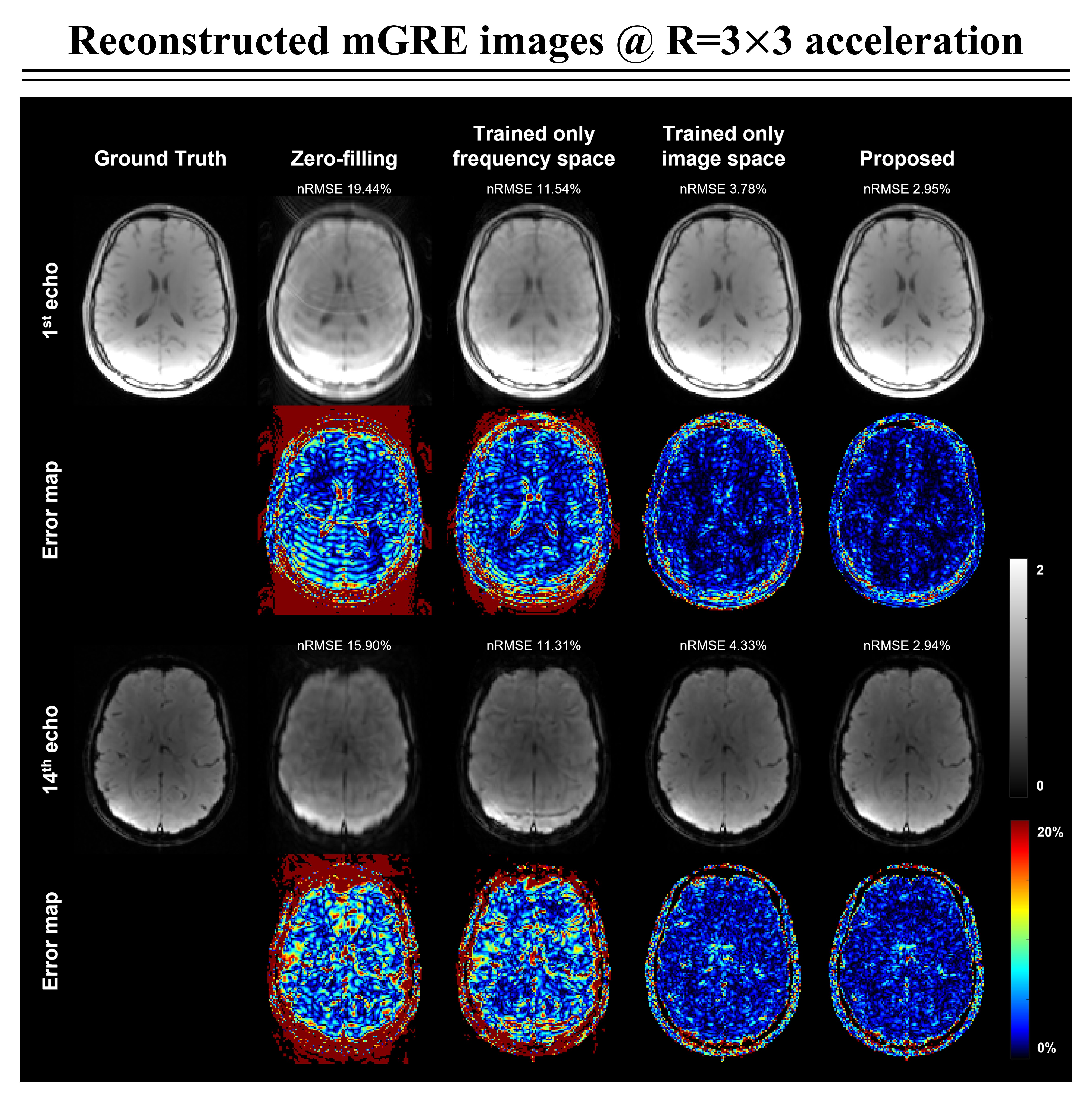
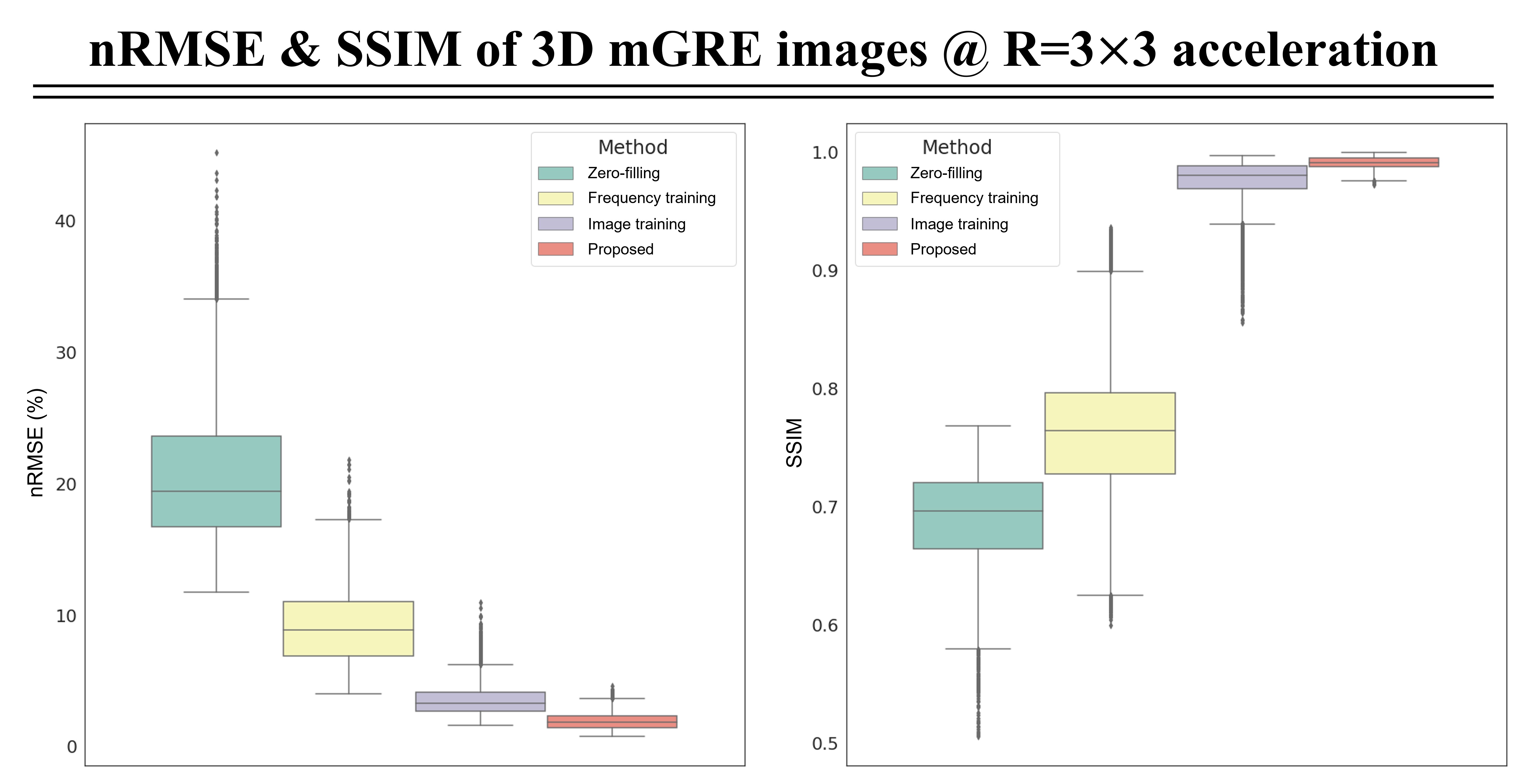
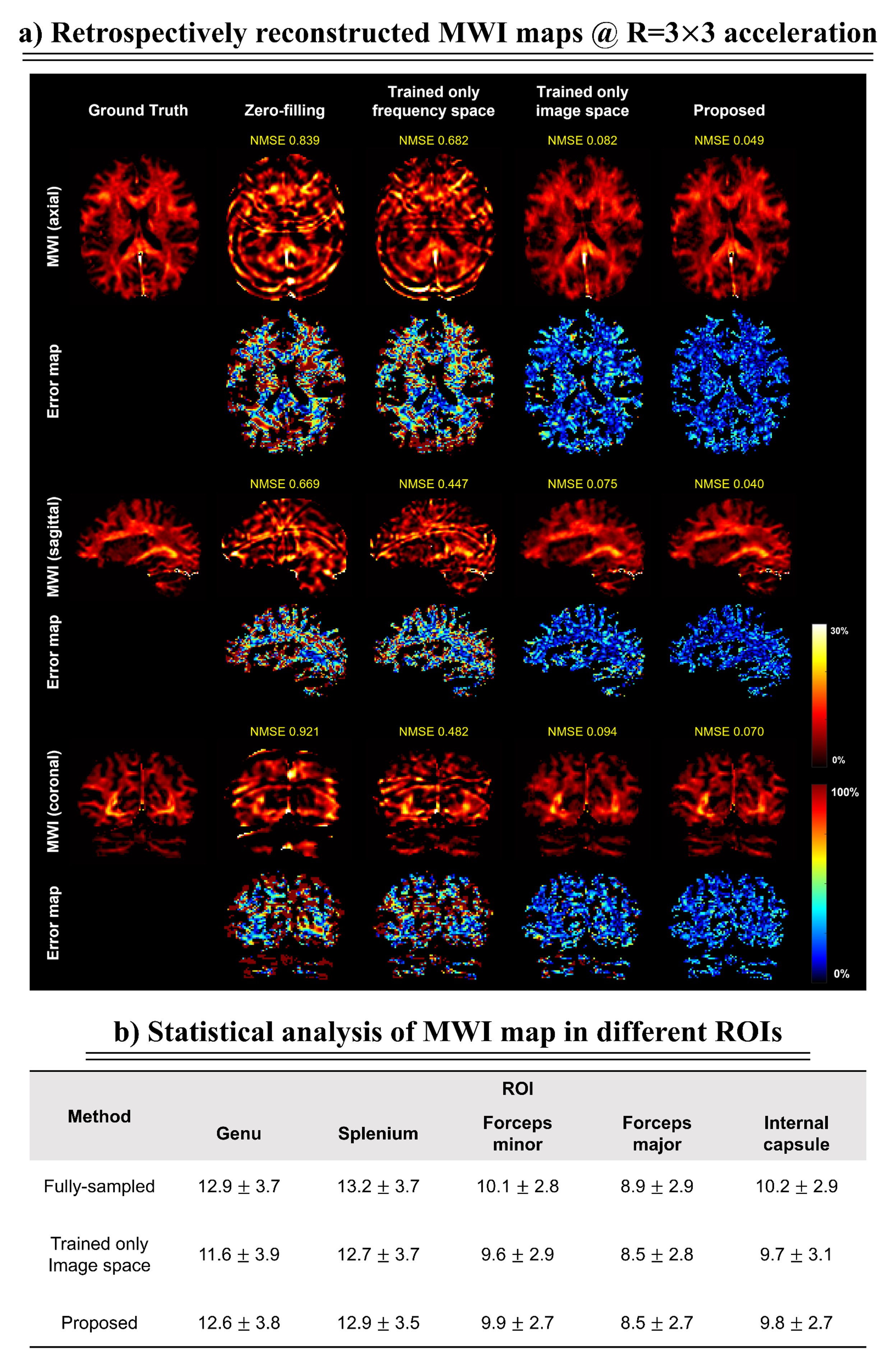
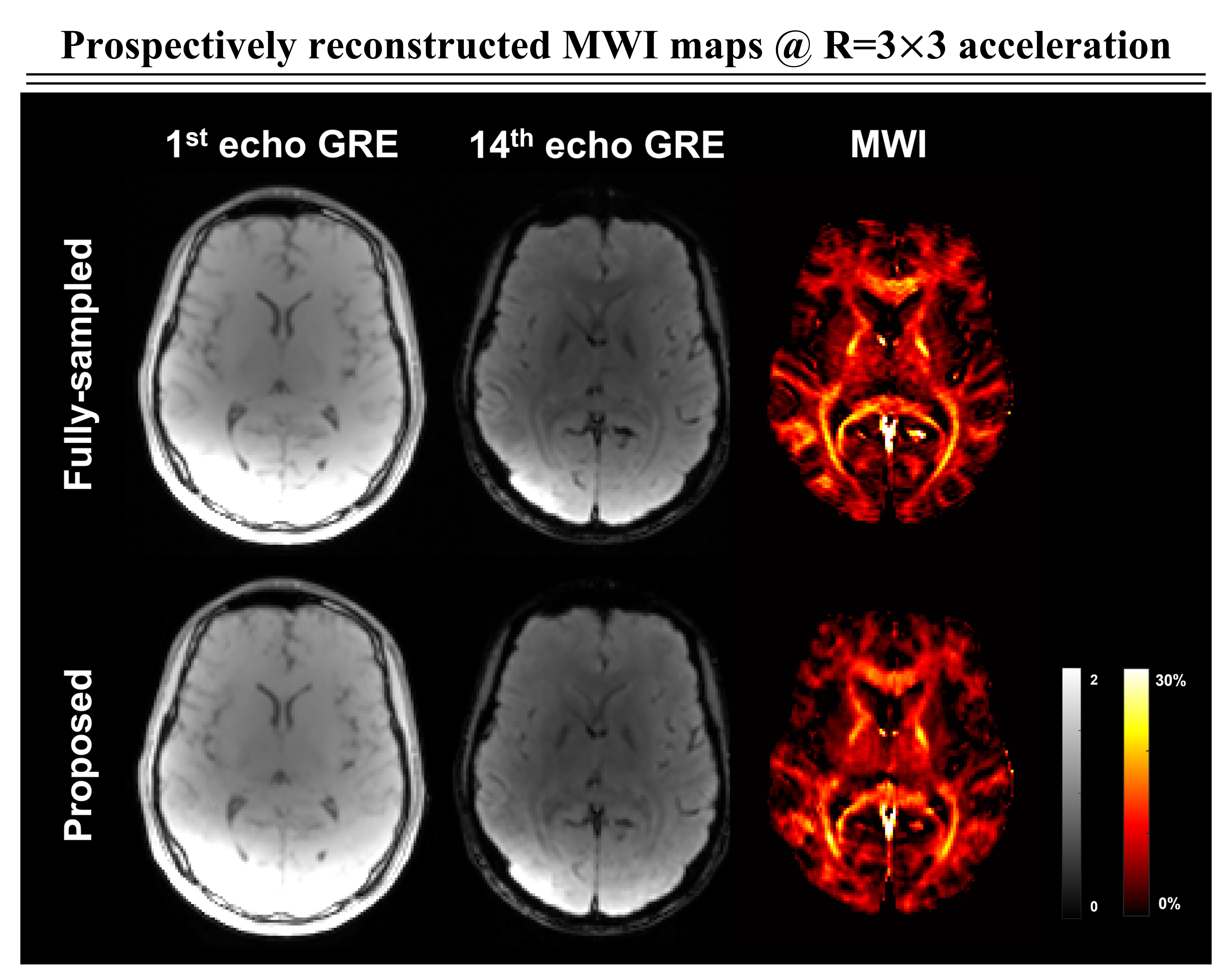
Figure 2 shows the comparative results of the reconstructed mGRE images using zero-filling, trained only on the frequency space, and trained only on the image space versus the proposed network. We illustrate the quantitative comparison of the normalized root-mean-square error (nRMSE) values and the structural similarity index (SSIM) scores of the reconstructed 3D mGRE images in Fig.3. The proposed method shows lower nRMSE values and higher SSIM scores than other comparative methods.
Figure 4a illustrates reconstructed MWI maps with the error maps. Quantitatively, the proposed method shows lower normalized mean-square error (NMSE) values compared to other methods with clear visualization. Figure 4b shows the local white matter regions of interest (ROIs) analysis. The prospectively reconstructed results show that the mGRE images and MWI maps of the prospective under-sampled data and fully-sampled data were highly similar (Fig.5). In addition, in the fully-sampled case, ringing artifacts can be seen due to the motion during the long scan time (15:23 minutes), which is mitigated in the prospective scan (2:22 minutes).

DISCUSSION AND CONCLUSION

In this work, we implemented a novel reconstruction network to accelerate 3D mGRE acquisition for the whole brain MWI map. We demonstrated the benefits of cross-domain optimization strategy with spatio-temporal decomposition. Additionally, the proposed architecture was designed to unroll the iterations of the reconstruction algorithms with the physics-inspired data consistency constraints (DC and WA blocks). The results indicate that the proposed network has potential advantages for correcting accelerated MRI data. Moreover, we exploited 2D+t spatio-temporal convolution layers to reconstruct independent GRE images and compensate for temporal T2* decay of mGRE images for MWI estimation. The proposed method could be feasible for accelerating 3D mGRE acquisition for MWI and clinical exam routines.

References

1. Mackay A, Whittall K, Adler J, et al. In vivo visualization of myelin water in brain by magnetic resonance. Magn Reson Med. 1994;31(6):673-677.
2. Lancaster J L., Andrews T, Hardies L. J, et al. Three-pool model of white matter. Journal of Magnetic Resonance Imaging. 2002;17(1):1-10.
3. Lee J-H, Yi J, Kim J-H, et al. Accelerated 3D myelin water imaging using joint spatio-temporal reconstruction. Med Phys. 2022;49(9):5929-5942.
4. Chen Q, She H, and Du Y P. Whole brain myelin water mapping in one minute using tensor dictionary learning with low-rank plus sparse regularization. IEEE Trans Med Imaging. 2021;40(4):1253-1266.
5. Li Y, Xiong J, Guo R, et al. Improved estimation of myelin water fractions with learned parameter distributions. Magn Reson Med. 2021;86(5):2795-2809.
6. Hwang D, Chung H, Nam Y, et al. Robust mapping of the myelin water fraction in the presence of noise: Synergic combination of anisotropic diffusion filter and spatially regularized nonnegative least squares algorithm. Journal of Magnetic Resonance Imaging. 2011;34(1):189-195.
7. Biyik E, Ilicak E, and Çukur T. Reconstruction by calibration over tensors for multi-coil multi-acquisition balanced SSFP imaging. Magn Reson Med. 2018;79(5):2542-2554.
8. Uecker M, Lai P, Murphy M J., et al. ESPIRiT-An eigenvalue approach to autocalibrating parallel MRI: Where SENSE meets GRAPPA. Magn Reson Med 2014;71(3):990-1001.
9. Ryu K, Lee J-H, Nam Y, et al. Accelerated multicontrast reconstruction for synthetic MRI using joint parallel imaging and variable splitting networks. Med Phys. 2021;48(6):2939-2950.
10. Singh N M., Iglesias J E, Adalsteinsson E, et al. Joint frequency and image space learning for MRI reconstruction and analysis. arXiv:2007.01441v3.
11. Jung S, Lee H, Ryu K, et al. Artificial neural network for multi-echo gradient echo-based myelin water fraction estimation. Magn Reson Med. 2020;85(1):380-389.