Synopsis

Keywords: Image Reconstruction, Machine Learning/Artificial Intelligence, Real-Time

Real-time MRI captures movements and dynamic processes in human body without reliance on any repetition or synchronization. Many applications require low-latency (typically <200ms) for guidance of interventions or closed-loop feedback. Standard constrained optimization methods are too slow to be implemented “online”. We demonstrate a non-Cartesian deep learning image reconstruction method based on the end-to-end variational network. Training data are created using traditional high latency compressed sensing reconstruction as the reference, with the goal of achieving similar results with low latency. We demonstrate reconstruction latencies of 95ms per frame, with nRMSE of 0.045 and SSIM of 0.95.

Introduction

The end-to-end variational network is a state-of-the-art deep learning method for static Cartesian image reconstruction [1]. In this work, we present a modified version to support RT-MRI applications that are both dynamic and non-Cartesian. The modifications include support for spiral data sampling, model-based sensitivity map estimation, a causal approach to the data consistency step, and weight sharing between cascades. We characterize reconstruction speed of the variational network and show much faster reconstruction than traditional iterative approaches [2].

Methods

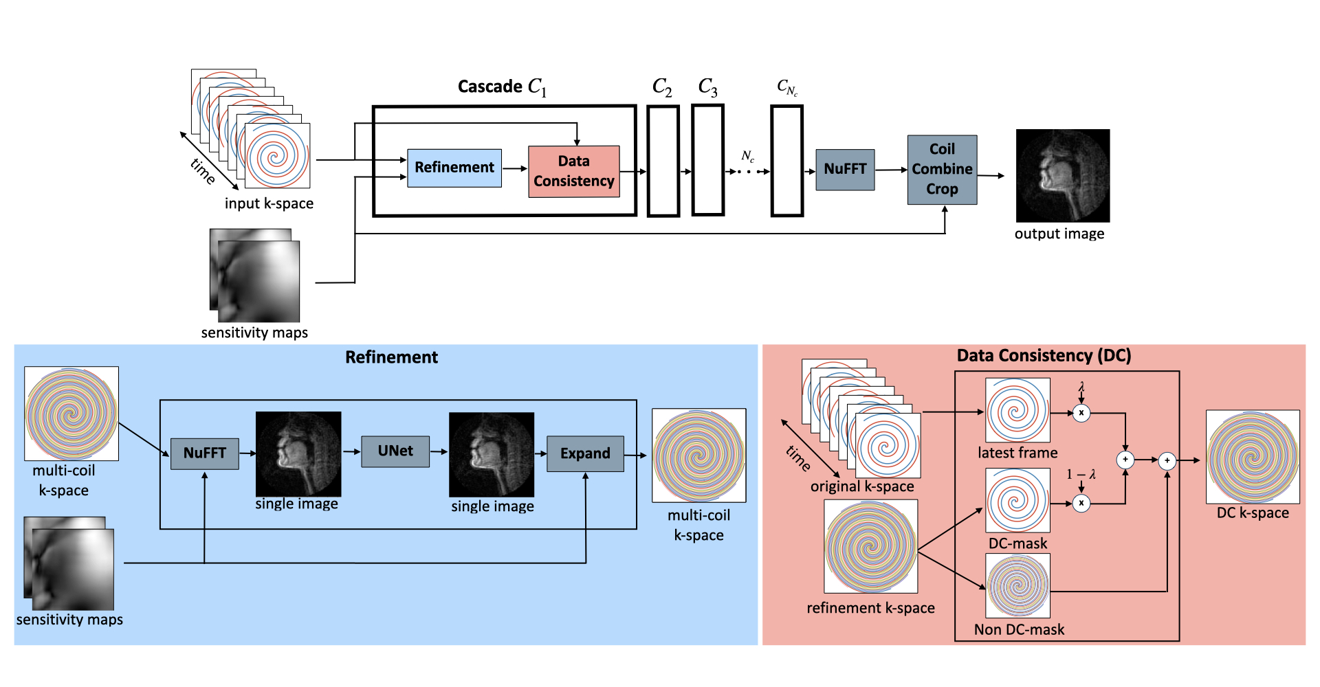
Figure 1 shows an overall flowchart of the method. Instead of FFT/IFFT operations for cartesian data, the “NuFFT adjoint with density compensation”/NuFFT was used for spiral data [3], [4]. We compute static coil sensitivity maps prior to the image reconstruction using the Walsh method [5] by averaging the entire dataset. To support a causal framework, we bin the latest fully sampled frames in a “view sharing” manner as an input to the network. In the data consistency (DC) step, we enforce only on the latest frame of k-space data (2 out of 13 interleaves). The model is trained both with or without weight sharing. The purpose of weight sharing is to aid interpretability by following a structure similar to iterative optimization approaches while decreasing the number of trainable parameters [6], [7].

The “75 speakers” dataset, a large dynamic vocal tract dataset, was used for training [8]. Each speaker has 32 speech tasks, amounting to 71,850 frames of data. The acquisition was a 13-interleaf spiral gradient echo at 1.5T. The ground truth reconstruction was an iterative constrained reconstruction with a temporal finite difference regularization, with an under-sample factor of 6.5. To keep training time reasonable, only ~1% of the dataset was used. The training set used 45 of the 75 speakers, using 3 of 32 randomly selected tasks from each subject and the middle 10% of each speaking task temporally.

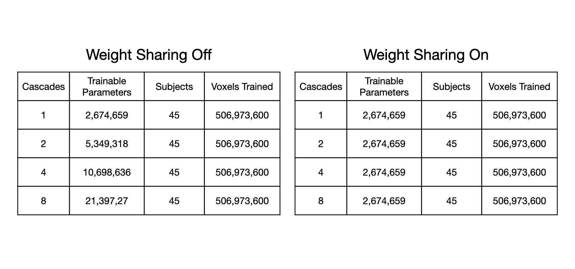
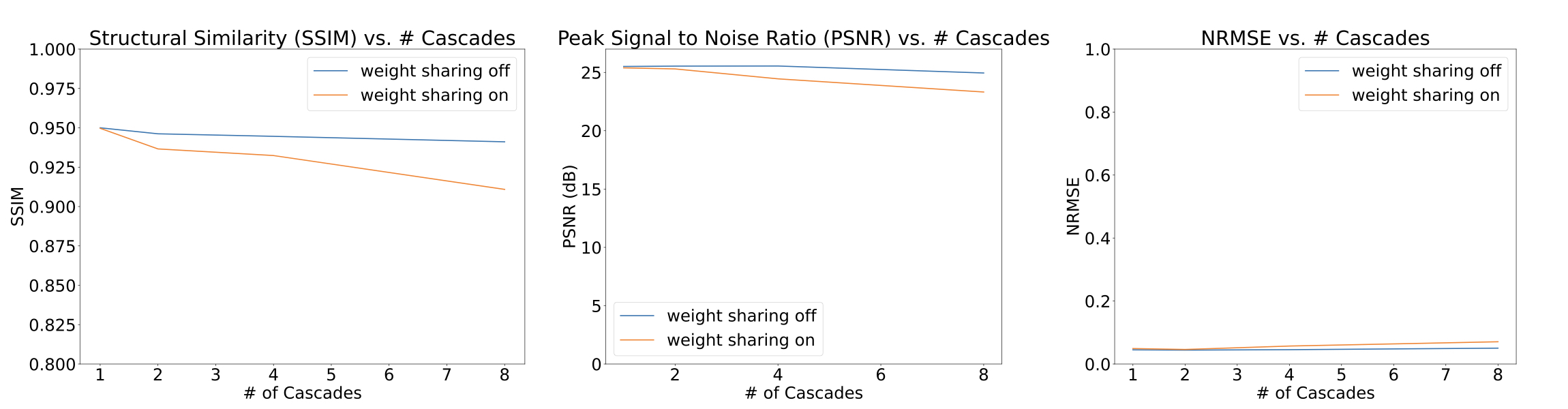
A trade-off analysis was conducted between number of cascades, image quality metrics, and inference time. We expected that as number of cascades increases, the increased number of trainable parameters should improve performance but would detriment inference time. Table 1 lists the number of trainable parameters without and with weight sharing. The metrics studied were structural similarity (SSIM), peak signal to noise ratio (pSNR), and normalized root mean-squared error (nRMSE).

The deep learning framework was implemented using Pytorch by modifying the end-to-end variational network provided in the fastMRI challenge [9]. The cost function minimized was the SSIM metric, using the ADAM optimizer. A batch size of 10 and learning rate of 0.001 was used. Training and inference were done with a Lambda Hyperplane compute-server and NVIDIA A100 GPU (40GB). For reproducibility, a full version of the code used will be shared prior to ISMRM.

Results

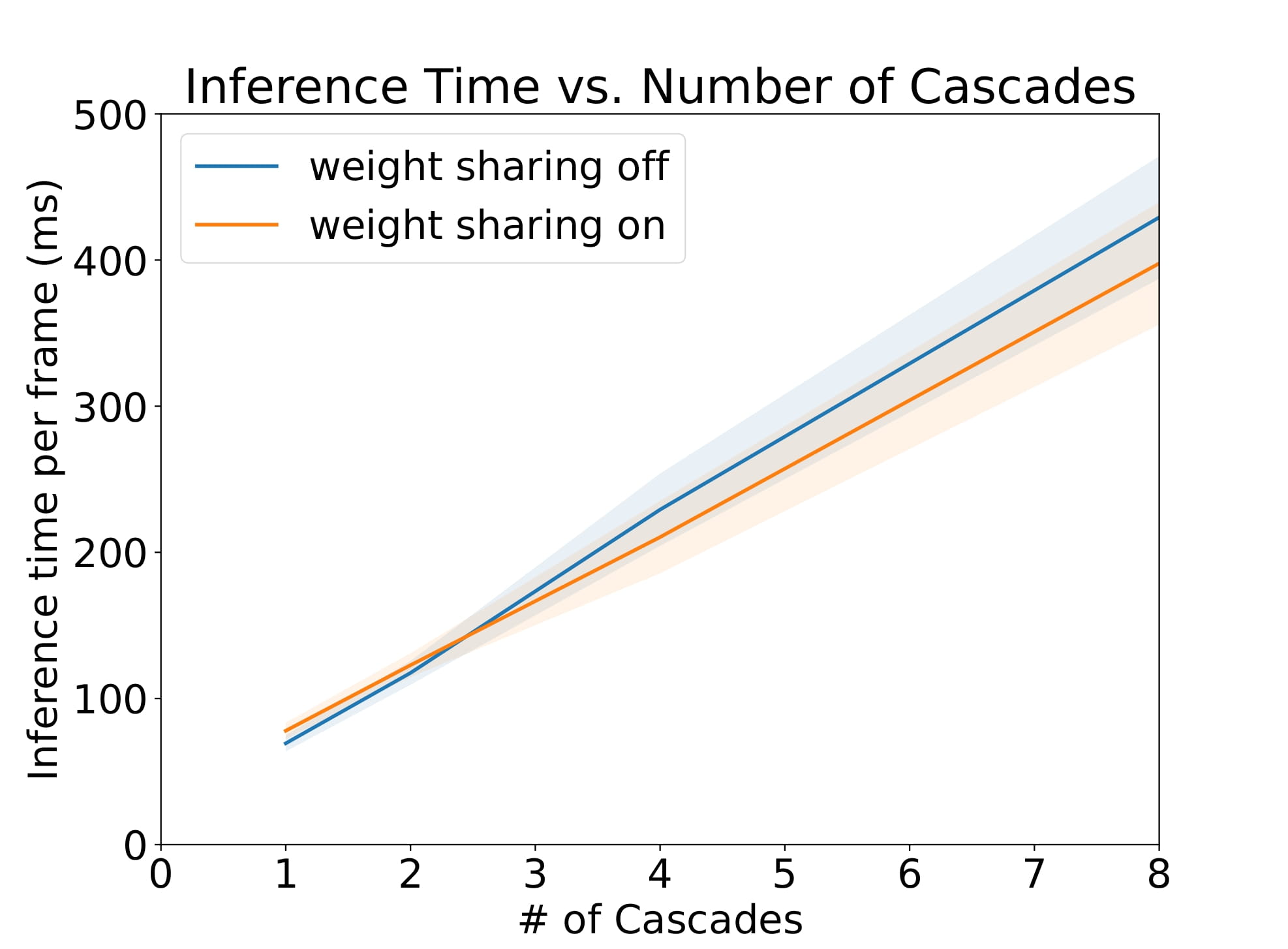
Figure 3 shows a plot of inference time vs number of cascades with and without weight sharing. Unsurprisingly, there is a linear relationship between the inference time and the number of cascades.

Figure 4 shows a plot of SSIM, PSNR, and MSE for the test set with various cascades both with and without view sharing. Surprisingly, as the number of cascades increases, the SSIM and PSNR decrease and the MSE increases.

Figure 5 shows intensity line profile of view sharing, ground truth, and variational network reconstructions, and shows that the deep learning network can reconstruct higher temporal resolution characteristics seen in the ground truth that cannot be recovered by simple view sharing.

Discussion

One cascade performed better than multiple cascades on all image quality metrics. This also provides incredibly short reconstruction times of around 100ms, which is fast enough for interactive applications.

We can think of many possible reasons as to why one cascade performed the best. First, there is inherent numerical instability in multiple calls to NuFFT adjoint with density compensation and NuFFT back again which cause irrecoverable artifacts. Multi-cascade blocks may cause extra instabilities with additional iterations, a problem the FFT/IFFT operation does not face after many iterations.

Second, the number of training samples was small and perhaps more is needed for the multiple cascade networks with a larger number of trainable parameters. Later work will include more training with the entire corpus of the 75 speakers’ dataset but was omitted for this study due to long training times (>1 week). However, it was experimentally found that adding new speakers to the training set had a much larger impact on test set performance than adding more speech tasks within the same subject, so using the entire corpus may contribute to overfitting to a specific set of subjects instead of improving performance.

In this work, we propose that in practice, sensitivity maps are computed and stored at the beginning of the scan session and used as an input to the network. An alternative to this is to use variable density spirals and jointly estimate sensitivity maps in an end-to-end manner such as in the E2E Variational Network [1]. This would require a new training dataset and remains future work.

Conclusion

We demonstrate low-latency (<100ms) image reconstruction of real-time dynamic MRI achieving similar reconstruction quality to compressed sensing iterative reconstruction methods.

Acknowledgements

We acknowledge grant support from the National Science Foundation (#1828736) and research support from Siemens Healthineers.