0821
Monotone Operator Learning: a robust and memory-efficient physics-guided deep learning framework1Electrical and Computer Engineering, University of Iowa, Iowa City, IA, United States
Synopsis
Keywords: Image Reconstruction, Machine Learning/Artificial Intelligence
MRI has been revolutionized by compressed sensing algorithms, which offer guaranteed uniqueness, convergence, and stability. In the recent years, model-based deep learning methods have been emerging as more powerful alternatives for image recovery. The main focus of this paper is to introduce a model based algorithm with similar theoretical guarantees as CS methods. The proposed deep equilibrium formulation is significantly more memory-efficient than unrolled methods, which allows us to apply it to 3D or 2D+time problems that current unrolled algorithms cannot handle. Our results also show that the approach is more robust to input perturbations than current unrolled methods.Introduction
Compressed sensing (CS) algorithms with theoretical guarantees on uniqueness, convergence and stability have made significant strides in parallel MRI (PMRI). Deep Unrolled (DU) optimization algorithms [1-4] are now outperforming CS algorithms both in performance and inference speed. A challenge with this scheme is the high memory demand during training time, which restricts the number of iterations, especially in high dimensional problems. In addition, these methods lack the above theoretical guarantees. Deep Equilibrium Networks (DEQ), which run the iterations to convergence, were introduced as memory efficient alternatives for DUs [5].We introduce a DEQ-based monotone operator learning (MOL) framework for PMRI recovery by constraining a residual CNN to be strictly monotone. We enforce monotonicity by constraining the Lipschitz constant of the CNN using a novel loss function (MOL-LR). MOL offers theoretical guarantees for uniqueness of solution, convergence and stability to perturbations, which are similar to CS methods; the proofs of these results are shown in our longer article [6]. Our experiments show that the proposed algorithm offers similar performance as DUs, while it is ten times more memory efficient. The higher memory efficiency allows us to apply it to 3D inverse problems. Our experiments also show that the algorithm is more stable to adversarial attacks.
Theory
The recovery of $$$\mathbf x \in \mathbb C^M$$$ from noisy under-sampled measurements $$$\mathbf b $$$ is formulated as, $$\mathbf x = \arg \min_{\mathbf x} \frac{\lambda}{2}\|\mathbf A(\mathbf x) - \mathbf b\|_2^2 + \phi(\mathbf x)$$ where $$$\mathbf A$$$ is a linear operator and $$$\phi(x)$$$ is an image prior. The estimate satisfies, $$\underbrace{\lambda \mathbf A^H (\mathbf A \mathbf x - \mathbf b)}_{ G(\mathbf x)} + \underbrace{\nabla \phi(\mathbf x)}_{ F(\mathbf x)} = 0. ~~~~(1)$$We constrain $$$F(x)$$$ as an $$$m$$$-monotone operator [4], which is satisfied when it can be represented as a residual CNN, $$ F = I - H_{\theta}, $$ where $$$H_{\theta} $$$ has a Lipschitz constant, $$ L[H_{\theta}] = (1-m); ~~0<m<1.$$ We use forward -backward splitting to obtain the MOL algorithm, $$\mathbf x_{n+1} = \underbrace{(I + \alpha \lambda \mathbf A^H \mathbf A)^{-1}\Big((1-\alpha)\mathbf x_n + \alpha H_{\theta}(\mathbf x_n) \Big)}_{T_{\rm MOL}(\mathbf x_n)} + \underbrace{( I + \alpha \lambda \mathbf A^H \mathbf A)^{-1}\Big( \alpha \lambda \mathbf A^H \mathbf b\Big)}_{\mathbf z}~~~(2) .$$
We use the above algorithm to realize a DEQ algorithm, where the algorithm is iterated to convergence. When the algorithm converges, the backpropagation steps can be evaluated using fixed point iterations, which is signficantly more memory efficient. We have the following theoretical results similar to CS algorithms [5]:
Uniqueness of fixed point: When $$$F$$$ is m-monotone, the fixed point specified by (1) is unique.
Convergence: For a fixed-point specified by $$$\mathbf x^*(\mathbf b)$$$, convergence of (2) is guaranteed when $$\alpha < \frac{2 m}{(2-m)^2} = \alpha_{\rm max} .$$
Robustness: Consider $$$\mathbf z_1$$$ and $$$\mathbf z_2$$$ to be measurements with $$$\boldsymbol\delta =\mathbf z_2-\mathbf z_1$$$ as the perturbation. If the corresponding MOL outputs are $$$\mathbf x^*(\mathbf z_1)$$$ and $$$\mathbf x^*(\mathbf z_2)$$$, respectively, with $$$\Delta= \mathbf x^*(\mathbf z_2)-\mathbf x^*(\mathbf z_1)$$$ as the output perturbation, $$ \|\Delta\|_2 \leq \frac{\alpha \lambda }{1-\sqrt{1 - 2\alpha m + \alpha^2(m-2)^2}}~\|\boldsymbol \delta\|_2.$$ When $$$\alpha$$$ is small, we have $$$\lim_{\alpha\rightarrow 0}\|\Delta\|_2 \leq \frac{\lambda}{m} \|\boldsymbol\delta\|_2$$$.
Training of MOL: For supervised learning, we propose to minimize $$ V(\theta) = \sum_{i=0}^{N_t} \|\mathbf x_i^* - \mathbf x_{i}\|_2^2 ~\mbox{s.t.}~ P\left(\mathbf x_i^*\right)\leq U; i=0,..,N_t $$ with respect to parameters $$$\theta$$$ of the CNN $$$\mathcal H_{\theta}$$$. Here, $$$U = 1-m$$$. The $$$\mathbf x_i; i=0,..,N_t$$$ and $$$\mathbf b_i, i=0,..,N_t$$$ are the ground truth images in the training dataset and their undersampled measurements, respectively. Here, $$$P\left(\mathbf x_i^*\right)$$$ is an estimate for the local Lipschitz constant [5].
Experiments and Results
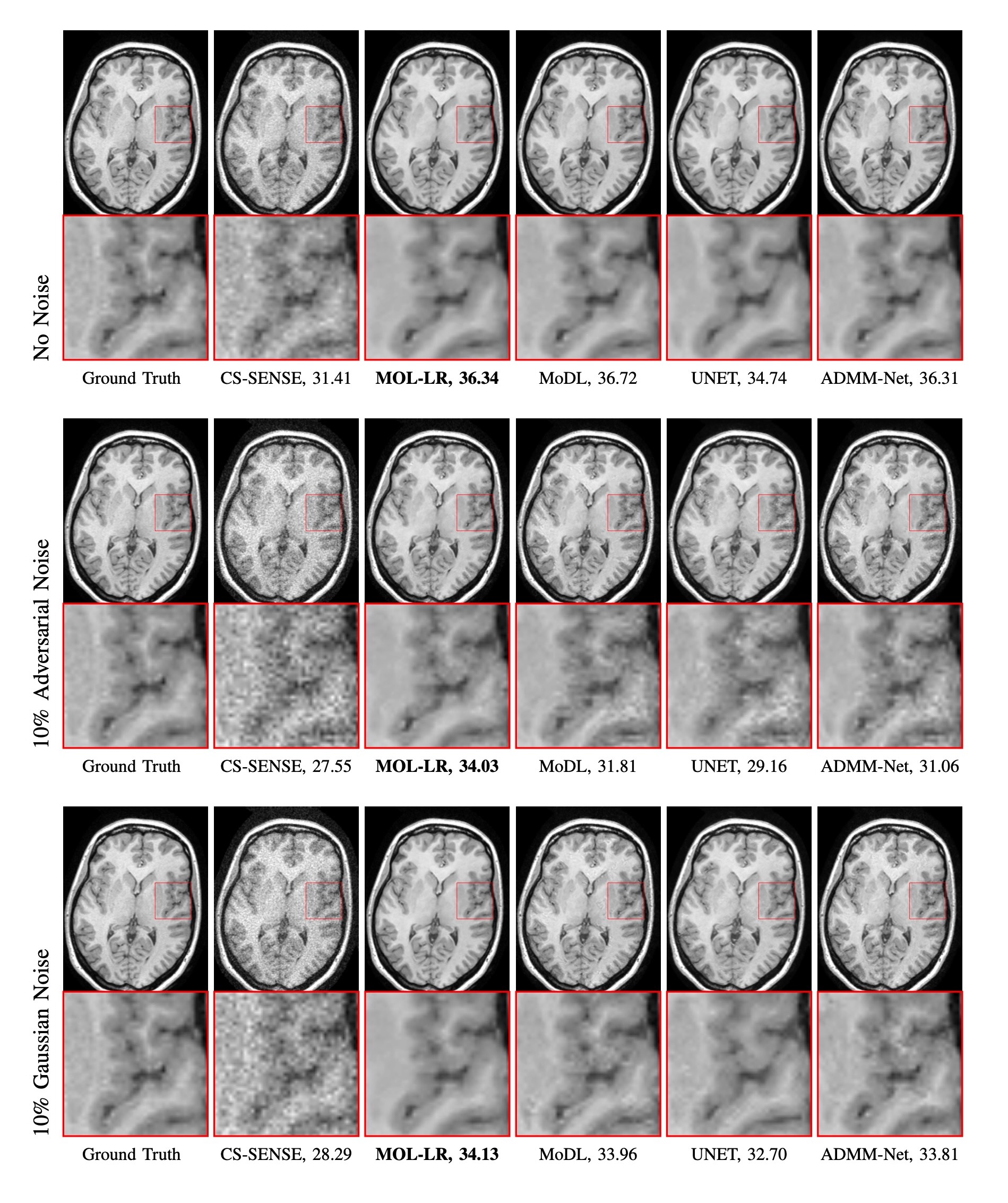
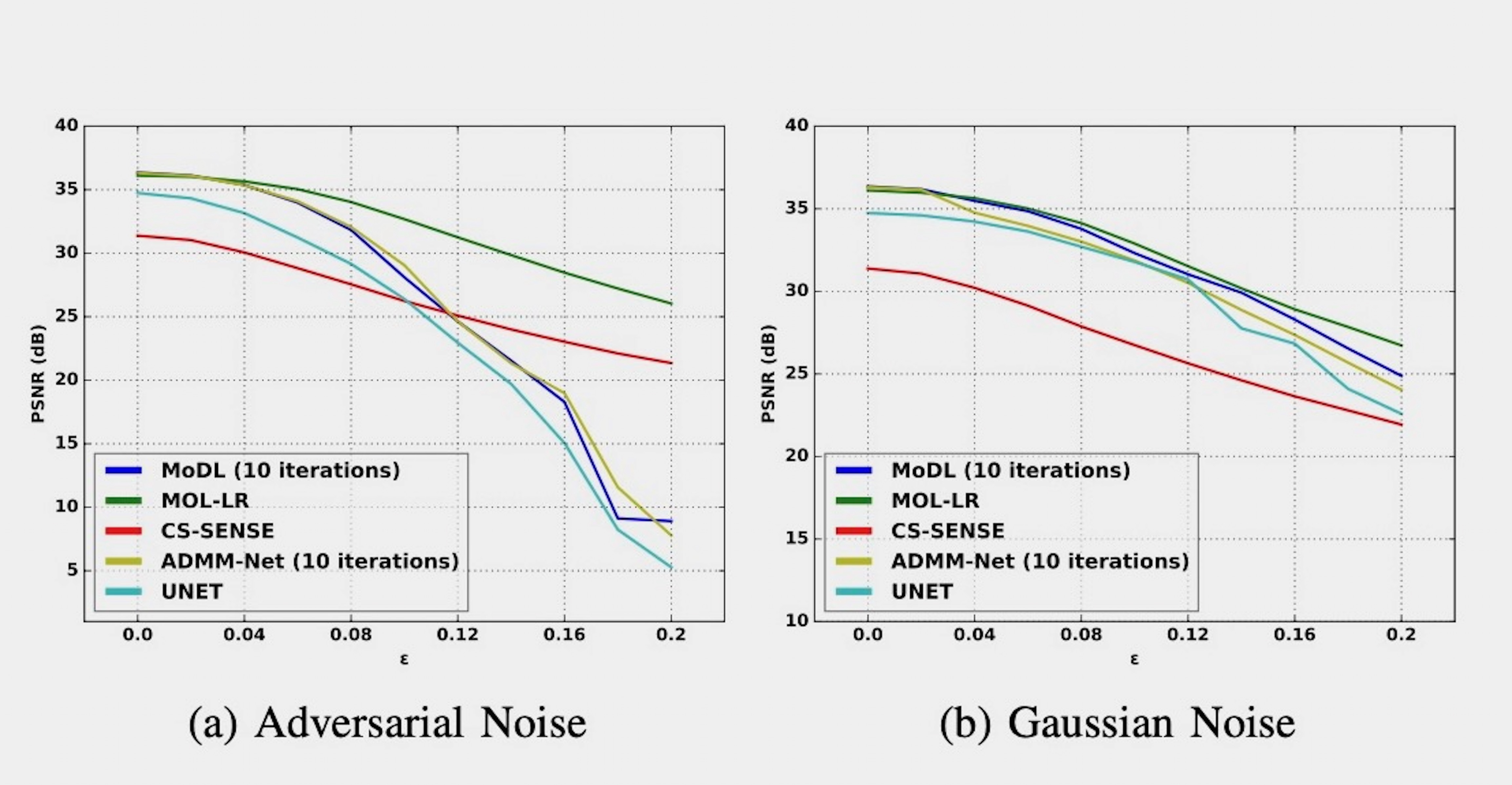
We perform experiments on publicly available Calgary Data [6]. It consists of 12-channel T1-weighted brain MRI. Data from 40, 7 and 20 subjects are split into training, testing and validation sets respectively. Cartesian 2D non-uniform variable density masks are used for 4-fold under-sampling of the datasets.Fig. 2 shows comparison of performance of MOL-LR against CS-SENSE [6], DUs MoDL [7] and ADMM-Net [8] and a CNN UNET [9]. We also compare the reconstructions when input is perturbed with 10% adversarial or Gaussian noise. With no additional noise, MOL-LR performs at par with MoDL and ADMM-Net. We note that the performance of both algorithms degrade linearly with Gaussian noise. However, the Lipschitz constrained MOL approach remain significantly less affected by adversarial perturbations compared to traditional unconstrained DUs (MoDL, ADMM-Net, UNET). Similar observations are also evident in the plots in Fig. 3.
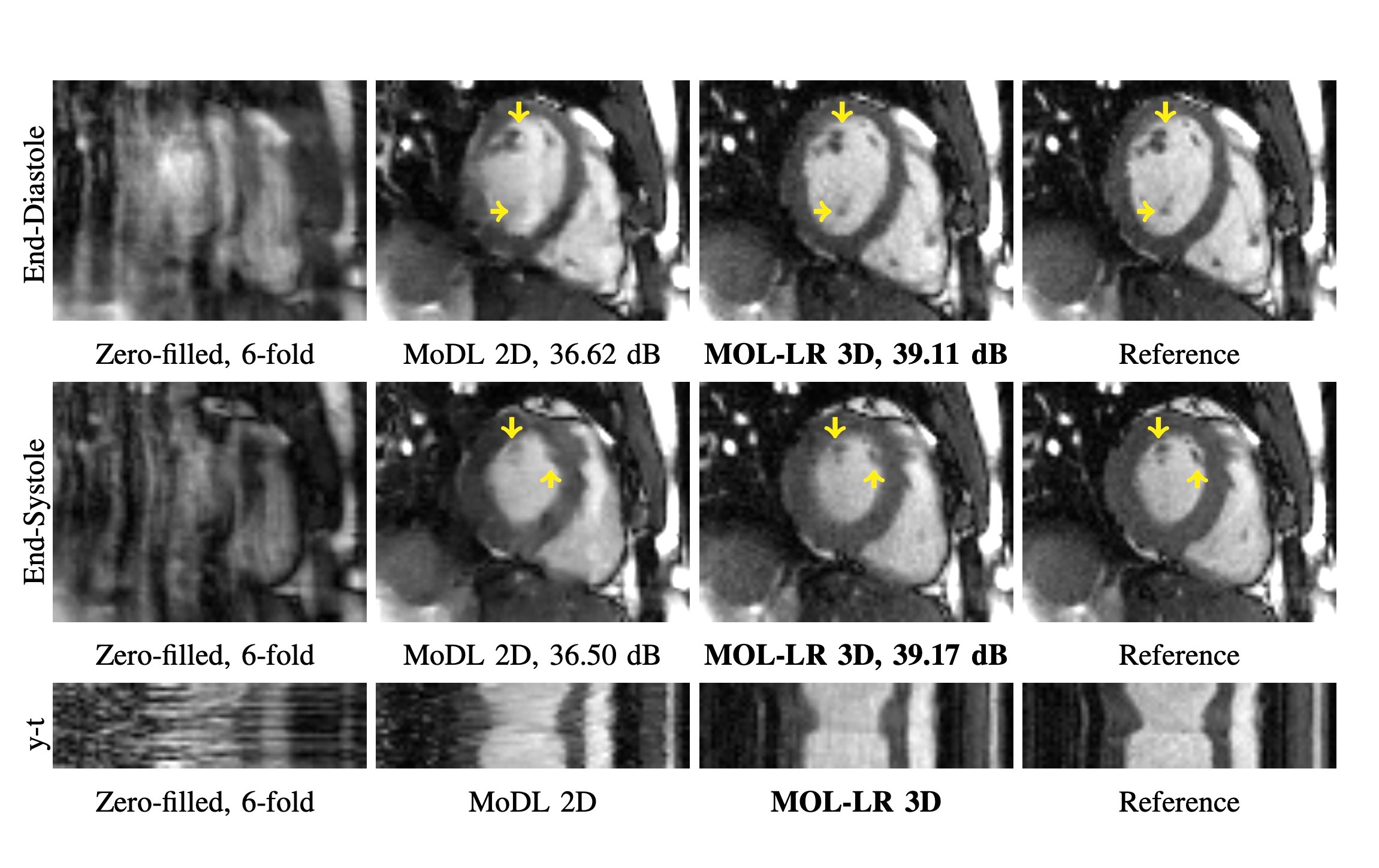
We demonstrate the benefit of memory efficiency in MOL through recovery of 6-fold under-sampled 2D+time cardiac data in Fig. 4. In a standard 16GB GPU, MoDL cannot fit multiple iterations for 2D+time data and hence performs 2D recovery instead. MoDL 2D is significantly outperformed by MOL-LR 3D in terms of PSNR. MoDL 2D suffers from lack of temporal information in 2D slices.
Conclusion
We introduced a DEQ based monotone operator learning framework for parallel MRI recovery. The framework comes with theoretical guarantees for uniqueness of solution, convergence and stability, similar to CS methods. Our experimental results show that it offers similar performance as DUs, which it has a ten fold lower memory demand. Experiments also show that the approach is more robust to worst-case input perturbations.Acknowledgements
This work is supported by NIH R01AG067078.References
[1] Hemant K. Aggarwal, Merry P. Mani, and Mathews Jacob. "MoDL: Model-based deep learning architecture for inverse problems." IEEE transactions on medical imaging 38.2 (2018): 394-405.
[2] Kerstin Hammernik, et al. "Learning a variational network for reconstruction of accelerated MRI data." Magnetic resonance in medicine 79.6 (2018): 3055-3071.
[3] Jian Sun, Huibin Li, and Zongben Xu. "Deep ADMM-Net for compressive sensing MRI." Advances in neural information processing systems 29 (2016).
[4] Jinxi Xiang, Yonggui Dong, and Yunjie Yang. "FISTA-net: Learning a fast iterative shrinkage thresholding network for inverse problems in imaging." IEEE Transactions on Medical Imaging 40.5 (2021): 1329-1339.
[5] Davis Gilton, Gregory Ongie, and Rebecca Willett. "Deep equilibrium architectures for inverse problems in imaging." IEEE Transactions on Computational Imaging 7 (2021): 1123-1133.
[6] Aniket Pramanik, and Mathews Jacob. "Stable and memory-efficient image recovery using monotone operator learning (MOL)." arXiv preprint arXiv:2206.04797 (2022).
Figures
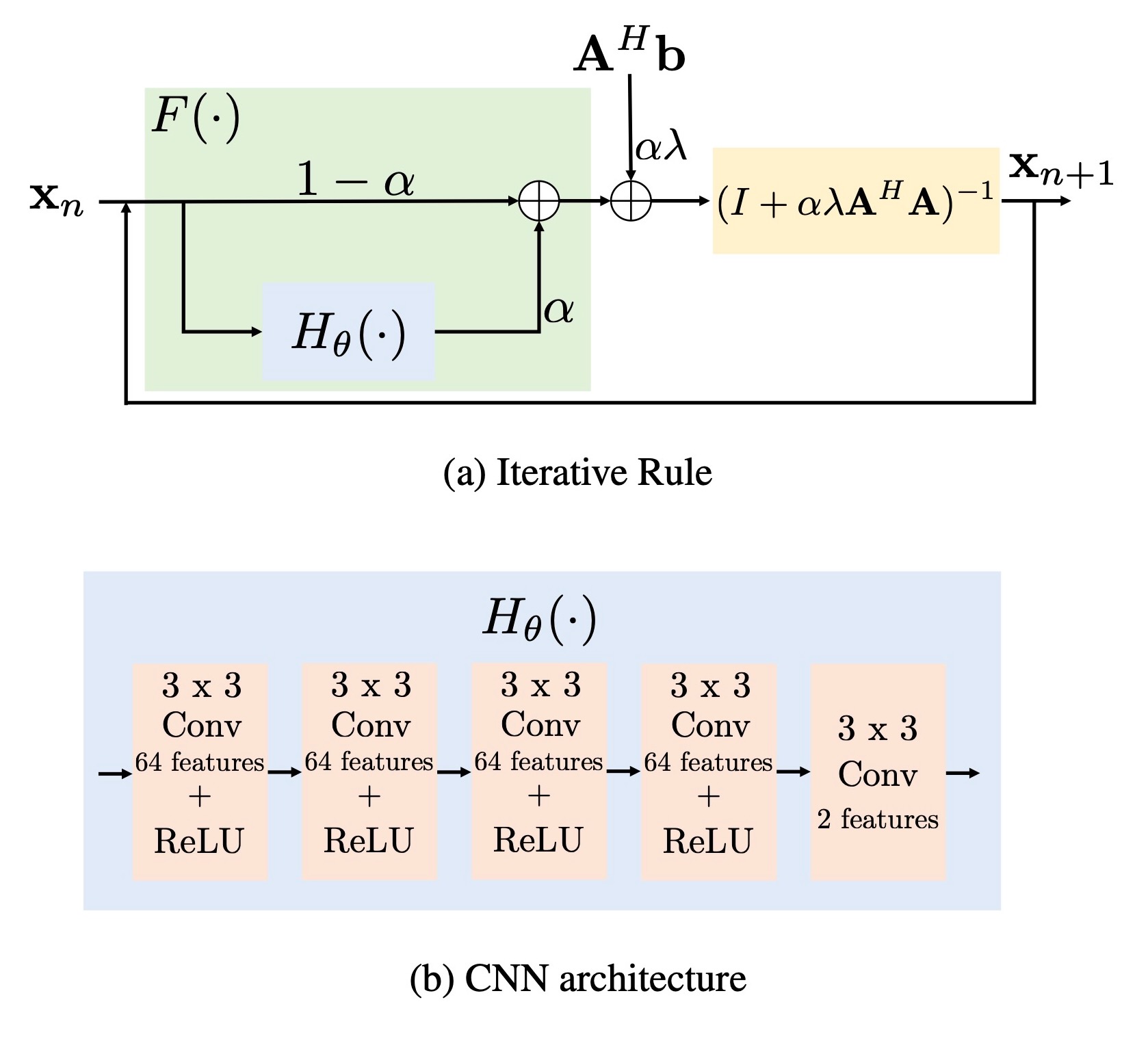
Fig. 1. Fig (a) shows fixed-point iterative rule of proposed MOL algorithm and (b) shows the architecture of the 5-layer CNN used in the experiments.