0767
No Wait Inversion – a novel model for T1 mapping from inversion recovery measurements without the waiting times
Anne Slawig1,2, Juliana Bibiano2, and Herbert Köstler2
1University Clinic and Outpatient Clinic for Radiology, University Hospital Halle (Saale), Halle (Saale), Germany, 2Department of Diagnostic and Interventional Radiology, University Hospital Würzburg, Würzburg, Germany
1University Clinic and Outpatient Clinic for Radiology, University Hospital Halle (Saale), Halle (Saale), Germany, 2Department of Diagnostic and Interventional Radiology, University Hospital Würzburg, Würzburg, Germany
Synopsis
Keywords: Signal Modeling, Relaxometry, T1 mapping, inversion recovery, model based reconstruction
This study proposes a combined fit of an inversion-prepared and non-prepared measurement for robust fast T1-mapping. Therefore, 24 slices in the brain were acquired with and without a global inversion pulse before each slice and no waiting time was heeded in between. Results of exponential model reconstructions for inversion measurement only, non-prepared measurement only and combined fitting of both measurements were compared towards their performance for T1-mapping. Robust and accurate T1-maps were achieved by the proposed combined model even in cases of imperfect inversion. It can thus eliminate long waiting times in between inversions or the necessity of perfect inversion pulses.Introduction
Recently, quantification of longitudinal relaxation time T1 became of interest as an important biomarker for tissue characterization. T1-mapping is employed in cardiac1–3 or brain imaging4–6.Standard inversion recovery measurements for T1-determination take prohibitively long and signal models assume a perfect inversion, which requires sophisticated, highly efficient inversion pulses to exclude errors7. Acceleration is possible by employing the Look-Locker technique or other accelerated, model-based algorithms8. But the calculation of real T1 values from Look-Locker acquisitions necessitates knowledge of equilibrium magnetization M0. Thus, usually a waiting time between global inversion pulses must be implemented to ensure complete relaxation of the tissue with the longest relaxation time before the next inversion. Also, high efficiency is demanded of inversion pulses as otherwise the M0 component can be corrupted, resulting in errors in the T1 estimation.
This study aims to introduce a novel model-based fitting approach for T1-mapping without the waiting times nor the necessity of perfect inversion pulses.
Methods
Two measurements (24 slices, TE=1.1ms, TR=9.3ms, flipangle=10°, resolution=0.8x0.8mm2, slice thickness=5mm, measurement time=4s for each slice) featuring a spiral readout were performed on a healthy volunteer at 3T(Siemens MAGNETOM PrismaFit). During one measurement no preparation and only slice-selective excitations were used. In the second measurement a global adiabatic inversion pulse was applied before the acquisition of each slice. No waiting time was heeded in between slices, and thus starting magnetization was affected by previous global inversion pulses. Both measurements acquire the course of the receiver coil weighted magnetization from a starting point (M0 or –δM0) to the steady state magnetization Mss.Initial images were reconstructed using a sliding window reconstruction, data was gridded and fitted using the corresponding exponential relaxation equations for
a) inversion recovery Look-Locker acquisition only: $$$M=Mss-(M0_1+Mss)*e^{(\frac{-t}{T1^*})}$$$
with 3 parameters(M01,Mss,T1*),
b) Look-Locker acquisition of non-inverted magnetization only: $$$M=Mss+(M0_2-Mss)*e^{(\frac{-t}{T1^*})}$$$
with 3 parameters(M02,Mss,T1*),
c) a combination of inverted and non-inverted Look-Locker acquisition
with 4 parameters(M01,M02,Mss,T1*).
Mss is the steady state magnetization, T1* the modified Look-Locker relaxation time9, M01 the equilibrium magnetization, determined as crossing point of y-axis, in non-prepared measurements and M02 the same in inversion-prepared measurements.
Absolute T1 values were calculated from fit parameters as: $$$T1=\frac{T1^**M0}{Mss}$$$7 and inversion efficiency as $$$InvEff=\frac{M0_1}{M0_2}$$$ from the combined model.
Results
Exemplarily, Figure 1 shows signal evolution and corresponding exponential fits. Note that combined fitting forces Mss and T1* to be similar for both relaxation processes, as data from identical tissue should feature identical tissue properties. Separate fitting imposes no such constraint.Figure 2 shows exemplary time points of both measurements. The inversion-prepared acquisition features the successive zeroing of different tissues.
Figure 3 shows parameter maps, as determined by the three different fit models. Mss is comparable in all cases. The non-prepared measurements suffer from low SNR and residual undersampling artifacts are visible in the map of the equilibrium magnetization M01, which hinders correct T1 calculation. Inversion recovery measurements enable robust fitting, but problems arise in cases of imperfect inversion or by altered magnetization due to the lack of waiting time between consecutive global inversions. The latter is especially apparent in tissues with long relaxation times like CSF, where M0 is determined unexpectedly low. Again, this considerably impacts T1 determination. In the combined fit two independent parameters (M01 and M02) are considered to allow for imperfect inversion and reduced initial magnetization. M02-maps show the effect of the reduced initial magnetization in tissue with long T1 times. But, as equilibrium magnetization is nicely determined by M01, robust T1 calculation is possible, as reflected in the detailed T1-map determined from parameters of the combined fit and T1-values corresponding to literature values10 (Table 1).
The efficiency of the inversion preparation is shown in Figure 4. Clearly, 100% inversion was not achieved in tissues with long relaxation time, but worked fine in other areas.
Discussion
The relaxation process from equilibrium magnetization (or inversion) into steady-state magnetization depends on T1 and can be fitted by corresponding exponential equation in inversion-prepared as well as non-prepared measurements. Main advantage of the former is the large dynamic range of signal evolution which benefits robust fitting especially in accelerated methods. But it also demands perfect inversion. By combining the inversion acquisition with a non-prepared measurement, M0 can be adequately recovered in a combined fit. Thus, no waiting time, or time consuming optimized inversion pulses, are necessary, as inversion does not need to be perfect. This is especially useful if global inversion pulses are used, as in simultaneous multi-slice imaging or 3D acquisitions. In this study total measurement time for all 24 slices was 192s for both measurements together. If the traditional waiting period of 5*T1 (approx. 4s in CSF) were observed, total measurement time would have been 556s, meaning an acceleration by the proposed algorithm by a factor of three. Further acceleration might even be possible by shortening the non-inverted acquisition. Also, through the combined fit model the performance of the inversion pulse can be investigated and is not a confounding factor for accurate T1-mapping anymore.Conclusion
The proposed model of a combined fit of an inversion-prepared and non-prepared measurement allows for robust fast T1-mapping, even in cases of imperfect inversion. It can thus render long waiting times in between inversion pulses redundant.Acknowledgements
No acknowledgement found.References
1. Kim PK, Hong YJ, Im DJ, et al. Myocardial T1 and T2 Mapping: Techniques and Clinical Applications. Korean J Radiol 2017;18:113–131 doi: 10.3348/kjr.2017.18.1.113.2. Taylor AJ, Salerno M, Dharmakumar R, Jerosch-Herold M. T1 Mapping: Basic Techniques and Clinical Applications. JACC: Cardiovascular Imaging 2016;9:67–81 doi: 10.1016/j.jcmg.2015.11.005.
3. Radunski UK, Lund GK, Stehning C, et al. CMR in patients with severe myocarditis: diagnostic value of quantitative tissue markers including extracellular volume imaging. JACC Cardiovasc Imaging 2014;7:667–675 doi: 10.1016/j.jcmg.2014.02.005.
4. Eminian S, Hajdu SD, Meuli RA, Maeder P, Hagmann P. Rapid high resolution T1 mapping as a marker of brain development: Normative ranges in key regions of interest. PLoS One 2018;13:e0198250 doi: 10.1371/journal.pone.0198250.
5. Deoni SCL, Peters TM, Rutt BK. High-resolution T1 and T2 mapping of the brain in a clinically acceptable time with DESPOT1 and DESPOT2. Magnetic Resonance in Medicine 2005;53:237–241 doi: 10.1002/mrm.20314.
6. Vrenken H, Geurts JJG, Knol DL, et al. Whole-Brain T1 Mapping in Multiple Sclerosis: Global Changes of Normal-appearing Gray and White Matter. Radiology 2006;240:811–820 doi: 10.1148/radiol.2403050569.
7. Kingsley PB, Ogg RJ, Reddick WE, Steen RG. Correction of errors caused by imperfect inversion pulses in MR imaging measurement of T1 relaxation times. Magn Reson Imaging 1998;16:1049–1055 doi: 10.1016/s0730-725x(98)00112-x.
8. Tran-Gia J, Wech T, Bley T, Köstler H. Model-Based Acceleration of Look-Locker T1 Mapping. PLOS ONE 2015;10:e0122611 doi: 10.1371/journal.pone.0122611.
9. Look DC, Locker DR. Time Saving in Measurement of NMR and EPR Relaxation Times. Review of Scientific Instruments 2003;41:250 doi: 10.1063/1.1684482.
10. Bojorquez JZ, Bricq S, Acquitter C, Brunotte F, Walker PM, Lalande A. What are normal relaxation times of tissues at 3 T? Magn Reson Imaging 2017;35:69–80 doi: 10.1016/j.mri.2016.08.021.
Figures
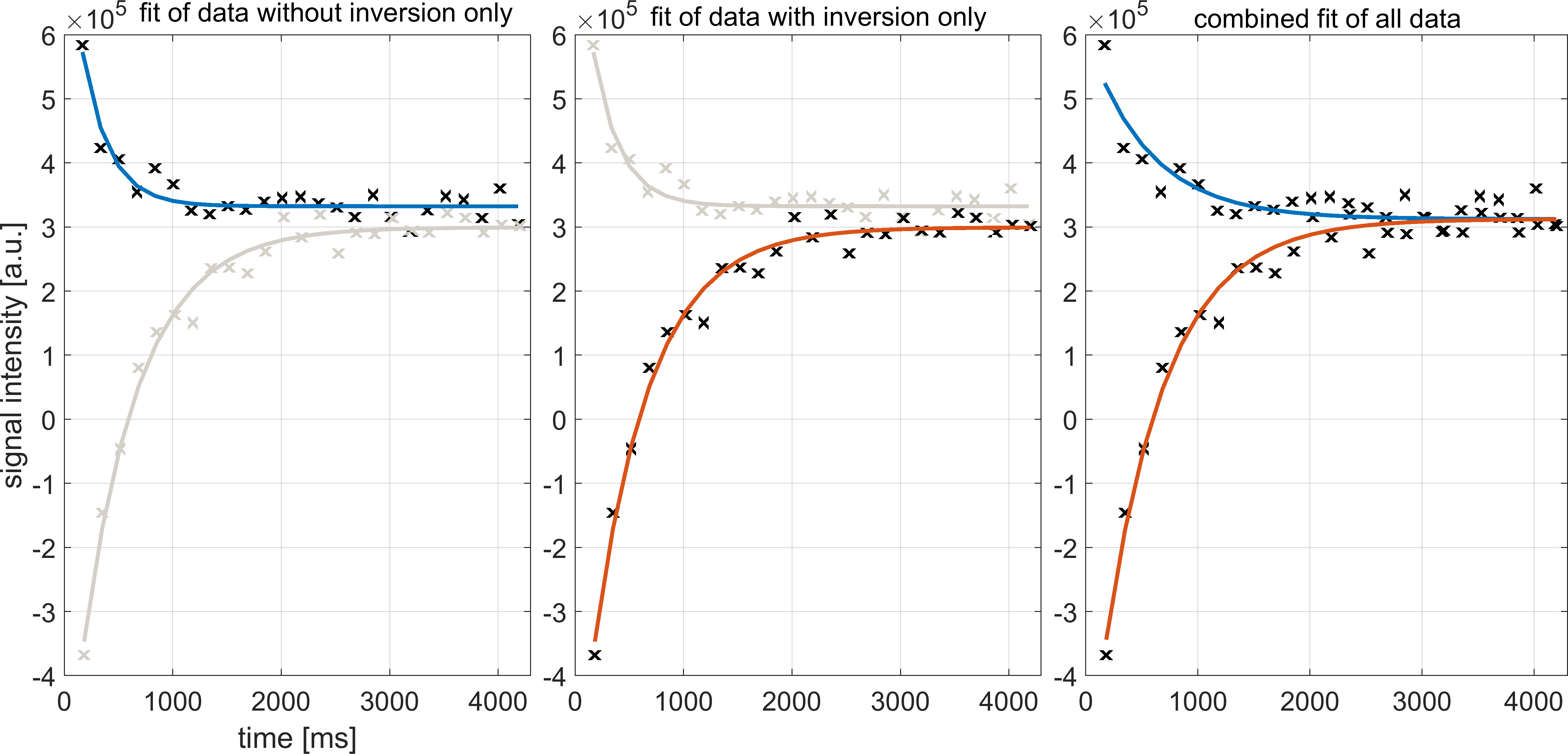
Figure 1: Comparison of the different fit models. Left: Fit of three parameters (Mss, M02, T1*) from one measurement without inversion only. Center: Fit of three parameters (Mss, M01, T1*) from one measurement with inversion only. Right: combined fit of four parameters (Mss, M01, M02, T1*) from both measurements. Note that combined fitting
forces Mss and T1* to be similar for both relaxation processes, as data from
identical tissue should feature identical tissue properties. Separate fitting imposes
no such constraint.
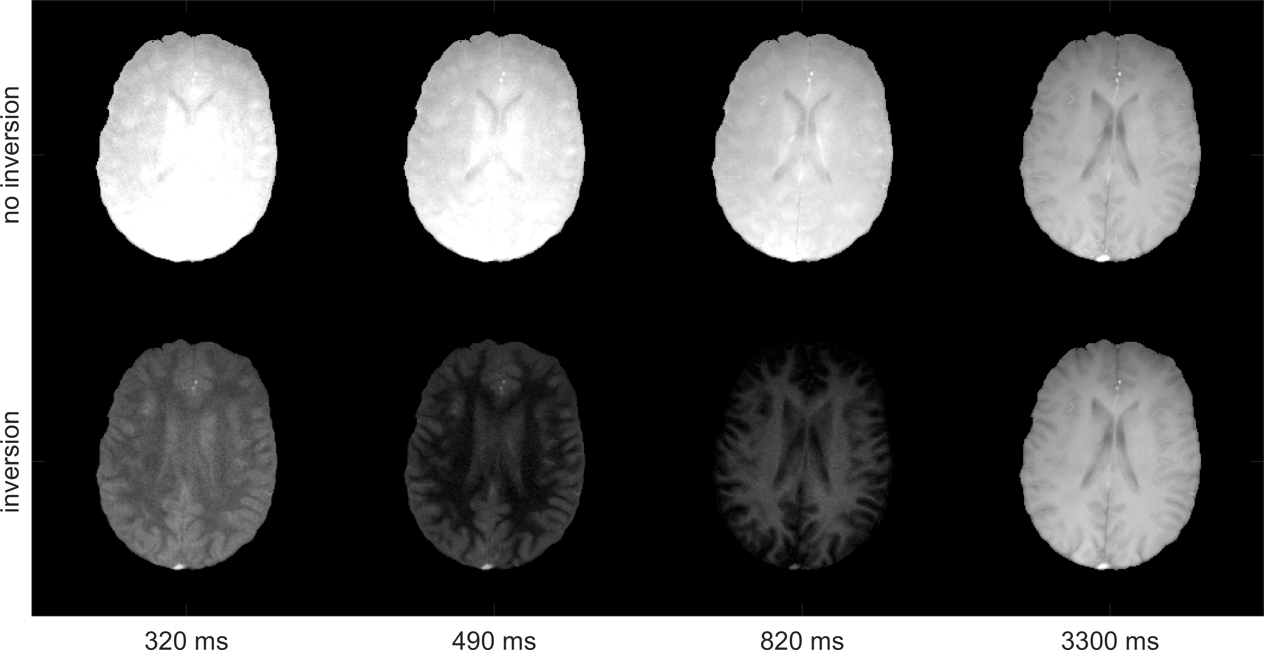
Figure 2: Exemplary time points from sliding window reconstruction of measurement without inversion (top) and measurement with inversion preparation (bottom). The inversion-prepared acquisition
features the successive zeroing of different tissues.
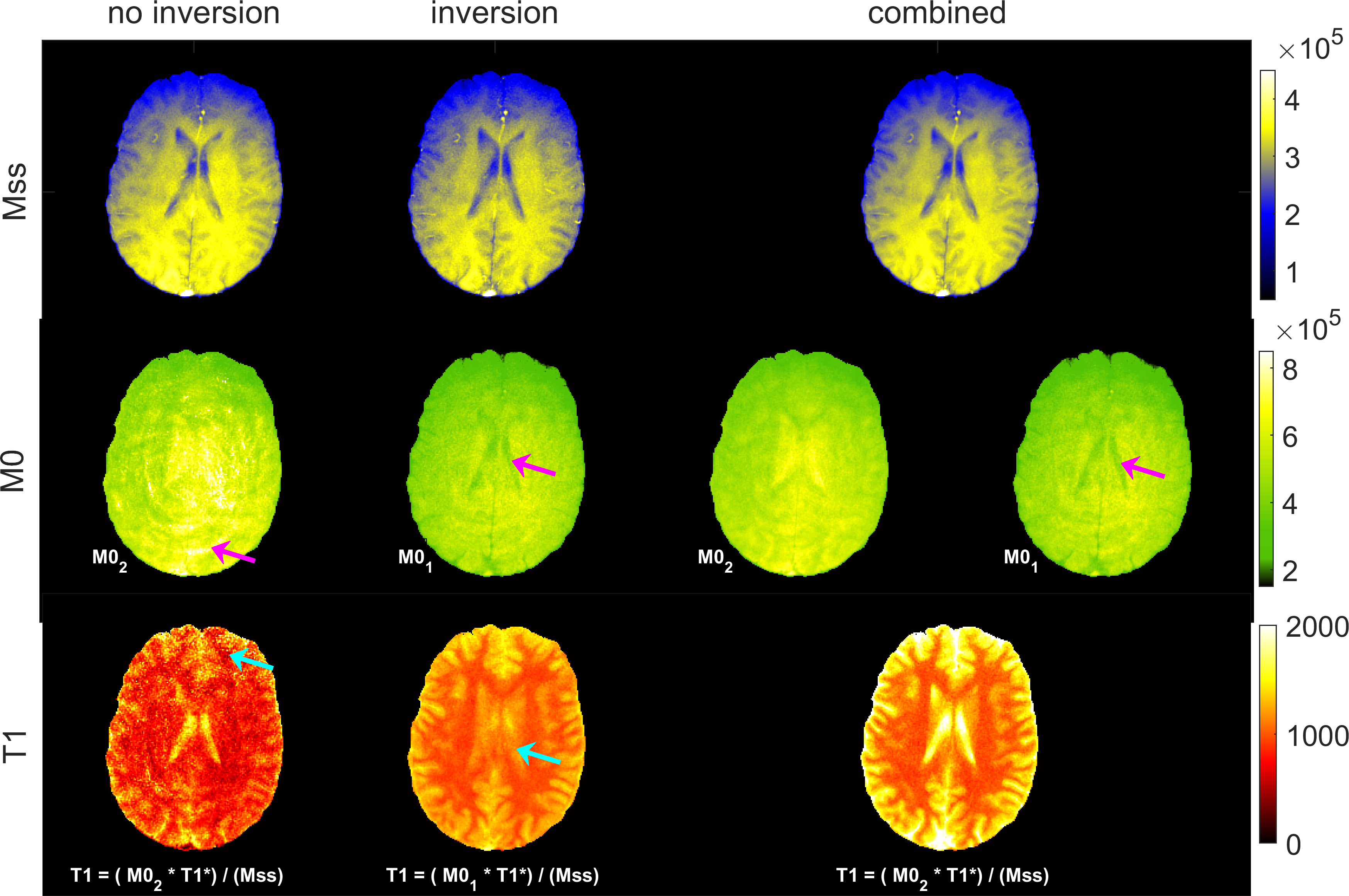
Figure 3: Parameter maps as determined by the three different fit models. Top: steady state magnetization (Mss). Center: equilibrium magnetization (M0). In the combined fit two independent parameters (M01 and M02) are considered to allow for imperfect inversion. Arrows point to problematic areas. Bottom: longitudinal relaxation times (T1) as calculated from fit parameters of data without inversion, with inversion and combined fit of both measurements. Blue arrows point to areas of obvious T1 underestimation.
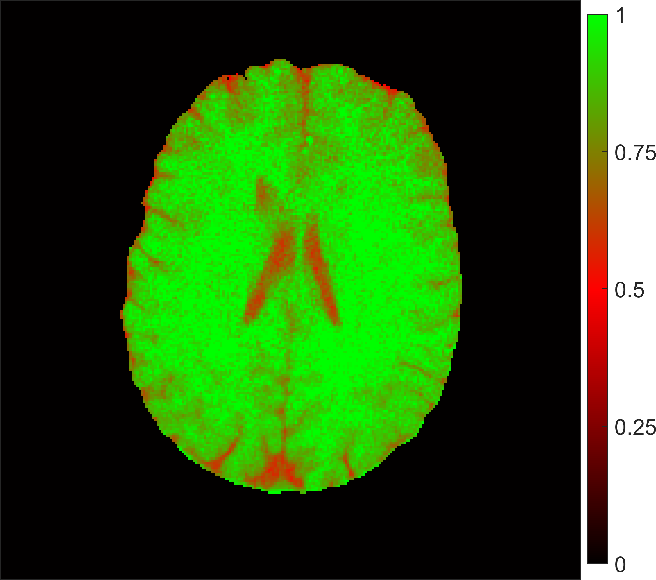
Figure 4: Inversion efficiency as determined of the ratio between the two parameters for M0 in the combined fit. Complete inversion was not achieved in
tissues with long relaxation time, but worked fine in other areas.
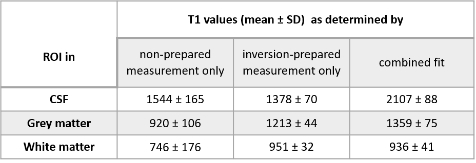
Table 1: T1 values (mean ± standard deviation) determined from ROIs placed in CSF, gray matter and white matter for all three different fitting approaches.
DOI: https://doi.org/10.58530/2023/0767