0763
Propagator-sensitive diffusion measurements hear the percussion ensemble
Evren Özarslan1, Deneb Boito1, and Alfredo Ordinola1
1Department of Biomedical Engineering, Linköping University, Linköping, Sweden
1Department of Biomedical Engineering, Linköping University, Linköping, Sweden
Synopsis
Keywords: Signal Modeling, Diffusion/other diffusion imaging techniques
In 1966, Kac asked the question ‘Can one hear the shape of a drum?’ which refers to linking the density of states function to the shape of the pores. We illustrate how the density of eigenstates as well as the pore shape can be obtained through diffusion measurements performed via a recently introduced arrangement of long and narrow gradient pulses. In the presence of dispersity, maps derived from the signal provide exquisite details about the ensemble of pore shapes within the voxel.Introduction
The cellular structure of tissues justifies envisioning them to be collections of isolated pores when the plasma membrane is sufficiently impermeable. In a recent work [1], it was demonstrated that the true diffusion propagator for a single closed domain can be reconstructed using a special arrangement of long and narrow gradient pulses (shown in Figure 1a), thus fully characterizing the diffusion process. Here, we illustrate two extensions of this method: (i) we show how the density of states function can be obtained from the detected signal, and (ii) we introduce new maps derived from the MR signal that provide exquisite details of the heterogeneous structure.Theory
The effective gradient waveform illustrated in Figure 1a enables one to reconstruct the diffusion propagator through the expression$$P(\mathbf{x}',\Delta|\mathbf{x}) =\frac{\int\mathrm{d}\mathbf{q}\, e^{i\mathbf{q}\cdot\mathbf{x}}\int\mathrm{d}\mathbf{q}'\, e^{i\mathbf{q}'\cdot\mathbf{x}'}\, E_\Delta(\mathbf{q},\mathbf{q}')}{(2\pi)^d \int\mathrm{d}\mathbf{q}\,e^{i\mathbf{q}\cdot\mathbf{x}}\, E_\Delta(\mathbf{q},\mathbf{0})}\ , \qquad(1)$$where $$$d$$$ is the number of dimensions, $$$P(\mathbf{x}',\Delta|\mathbf{x})$$$ is the propagator, and $$$E_\Delta(\mathbf{q},\mathbf{q}')$$$ is the signal attenuation.The eigenfunction expansion of the propagator can be used to obtain the following expression:$$\int\, P(\mathbf{x},t|\mathbf{x}) \, \mathrm{d}\mathbf{x} = \int\,p(\lambda)\,e^{-\lambda t}\,\mathrm{d}\lambda \qquad(2),$$Let $$$W_\Delta(\mathbf{x},\mathbf{x}’)$$$ indicate the two-dimensional inverse Fourier transform of $$$E_\Delta(\mathbf{q},\mathbf{q}')$$$. We introduce a suite of new quantities in Figure 1b.Methods
A simulation framework employing the multiple correlation function (MCF) [2] approach was implemented in Python. Signals from a single slab of size $$$5\mu\,m$$$ with hard reflecting walls were computed for $$$51\times51$$$ different (q,q’) combinations and 300 diffusion times $$$t$$$ for the sequence in Figure 1a. The q-values ranged from $$$-4$$$to$$$+4\mu\,m^{-1}$$$, and the diffusion times from $$$0.001$$$to$$$3ms$$$. The quantity $$$P(x',t|x)$$$ was then computed for all times through Equation 1 as well as the left-hand side of Equation 2 through a simple numerical integration. Finally, $$$p(\lambda)$$$ is obtained through a numerical implementation of the inverse Laplace transform provided at https://github.com/caizkun/pyilt/).The maps of the quantities in Figure 1b were computed from the long time diffusion measurements for the different collections of compartments. For each collection, 5000 geometries were defined on 2-dimensional grids using both cartesian and polar coordinates. Both grids were composed of 151 intervals in each dimension. Each geometry was created so that its center of mass would be located at the origin of the grid. Computations of $$$\bar{\rho}$$$ and $$$\sigma_g$$$ were carried out on the geometries defined on the cartesian grid, while computations of $$$\Phi$$$ were carried out on the same geometries defined in polar coordinates.
Results
Different steps in the extraction of $$$p(\lambda)$$$ from simulated data are presented in Figure 2, featuring the signal decay for all (q,q’) combinations at three different diffusion times, the computed diffusion propagators, the left-hand side of Equation 2, and $$$p(\lambda)$$$.In Figures 3-5, we show the maps of the quantities provided in Figure 1b for collections of compartments with different features.
Discussion & Conclusion
The reconstructed density of states $$$p(\lambda)$$$ is in good agreement with the expected location of peaks for the first few terms. However, as the frequency of states increases, the spectrum converges to a continuous curve from which single peaks are complicated to resolve. Nevertheless, it is encouraging to observe distinct states for the simulated geometry with a small pore size with the first realization of this framework.The quantitative maps illustrated in Figures 3-5 provide sufficient information to characterize and distinguish all collections of compartments considered. Compared to earlier methods that rely on simple scalar metrics, the introduced quantities provide much more information on the morphological properties of the compartments making up the specimen.
In 1966, Kac posed the question ‘Can one hear the shape of a drum?’ which concerns a possible link between the density of states function and the shape of the pores [3]. Earlier work [4] had demonstrated how the shape of a drum can be measured via magnetic resonance. Here, we showed how magnetic resonance hears a drum or even a percussion ensemble.
Acknowledgements
No acknowledgement found.References
[1] E. Özarslan. Recovering almost everything diffusion could reveal, in Proc Intl Soc Mag Reson Med, 29, 2021, p. 3637.
[2] D. S. Grebenkov. NMR survey of reflected Brownian motion. Rev Mod Phys. 2007;79(3):1077-1137.
[3] M. Kac, Can one hear the shape of a drum?, Am Math Mon 73, 1 (1966).
[4] F. B. Laun, T. A. Kuder, W. Semmler, and B. Stieltjes, Determination of the defining boundary in nuclear magnetic resonance diffusion experiments, Phys Rev Lett 107, 048102 (2011).
Figures
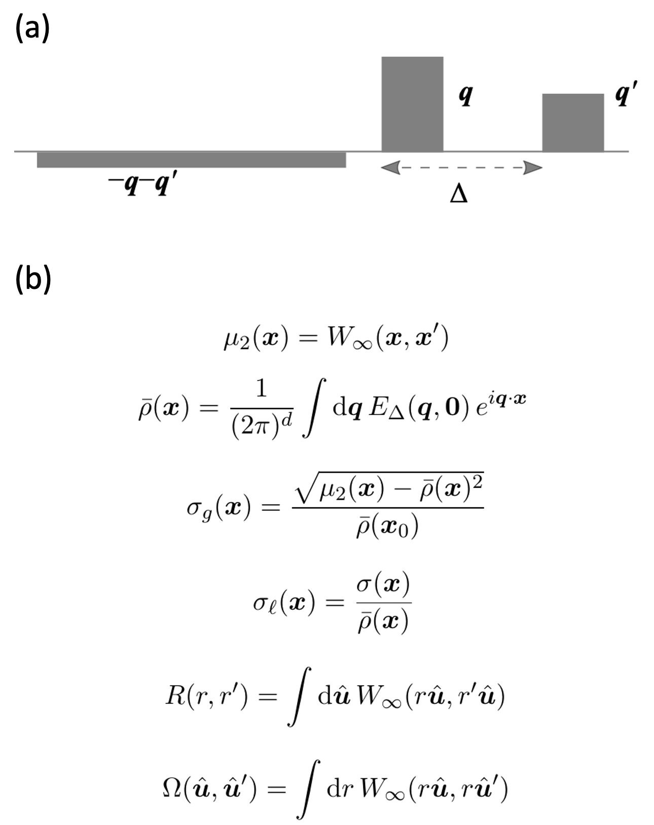
(a) The effective waveform for the propagator-sensitive measurement introduced in [1]. The gray boxes indicate gradient pulses. (b) New measures we introduce for characterizing dispersity.
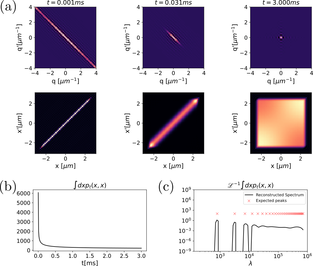
Different steps in the reconstruction of $$$p(\lambda)$$$ of a single pore from simulated signals obtained from the proposed pulse sequence in [1]. (a) Top: signal decay for three diffusion times. Bottom: computed $$$p_t(x,x’)$$$ for the same times. (b) Left-hand side of Equation 2. (c) Reconstructed spectrum $$$p(\lambda)$$$, and expected position of delta-dirac functions $$$\lambda_n$$$.
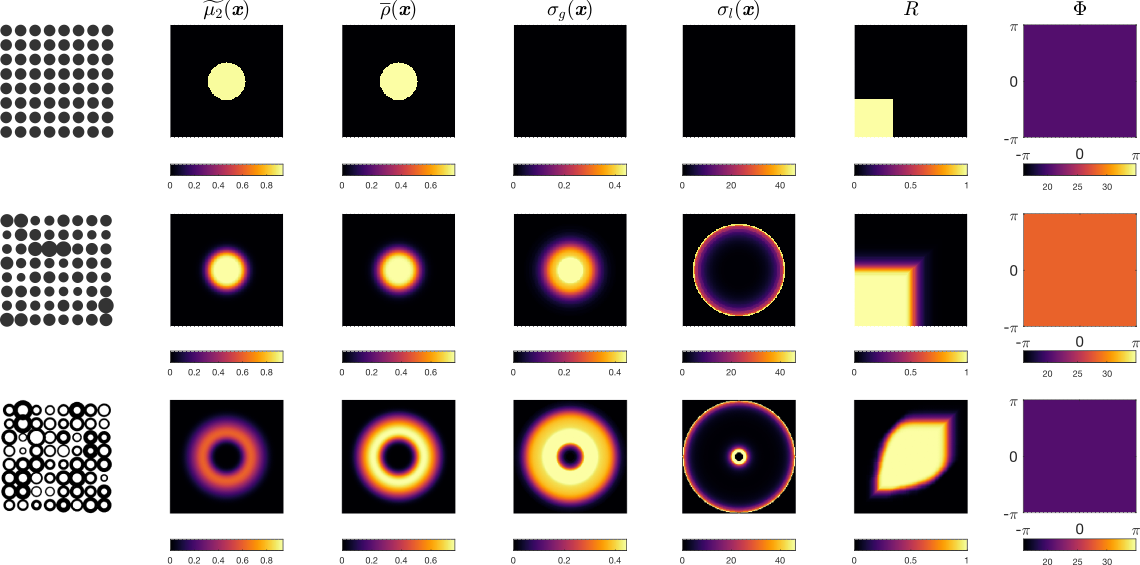
Maps computed from the long-time diffusion measurements for different specimens comprising isotropic compartments.
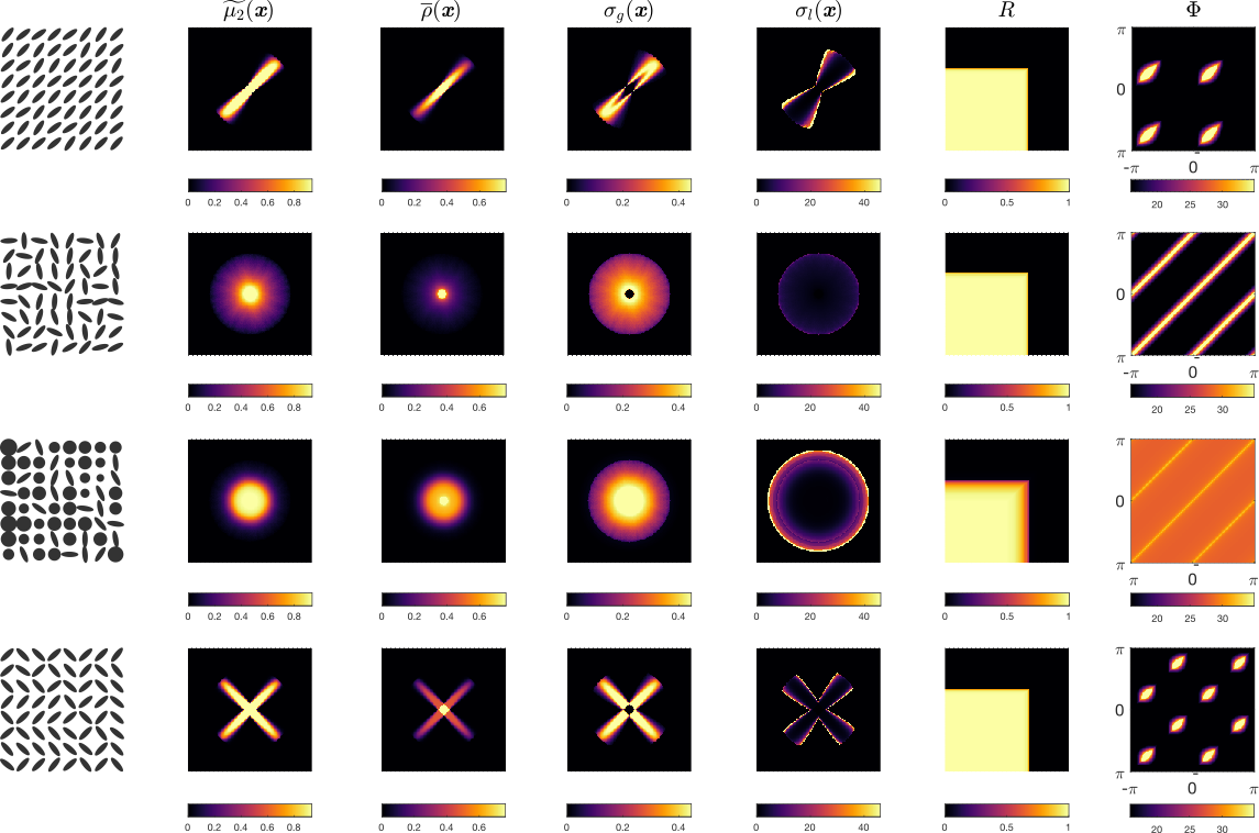
Maps computed from the long-time diffusion measurements for different specimens comprising anisotropic compartments.
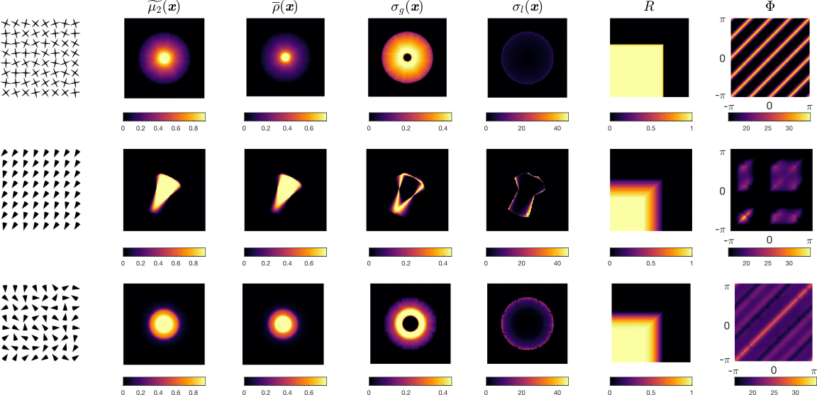
Maps computed from the long-time diffusion measurements for different specimens comprising plus-shaped and asymmetric compartments.
DOI: https://doi.org/10.58530/2023/0763