0759

Quasi-Diffusion: A Model Of Signal Attenuation In Diffusion Magnetic Resonance Imaging Of Brain Tissue

Thomas R Barrick¹, Carson Ingo^2,3, and Franklyn A Howe¹
¹Department of Neurosciences, St George's, University of London, London, United Kingdom, ²Department of Neurology, Northwestern University, Chicago, IL, United States, ³Department of Physical Therapy, Human Movement Sciences, Northwestern University, Chicago, IL, United States

Synopsis

Keywords: Signal Modeling, Diffusion/other diffusion imaging techniques

We show the quasi-diffusion model describes the dMRI signal from low b-value (stretched exponential) to high b-value (power law) regimes via a single, parsimonious function of two independent parameters. We identify new tissue contrast via a signal inflection point indicating the transition to the localisation regime. Quasi-Diffusion Imaging (QDI) parameter estimates converge to stable values as maximum b-value is increased, suggesting quasi-diffusion is a valid model for brain tissue dMRI signal decay. Accuracy of QDI parameters computed from 4 b-values of a 12 b-value acquisition indicate QDI measures may be derived from data acquired in clinically feasible times.

Introduction

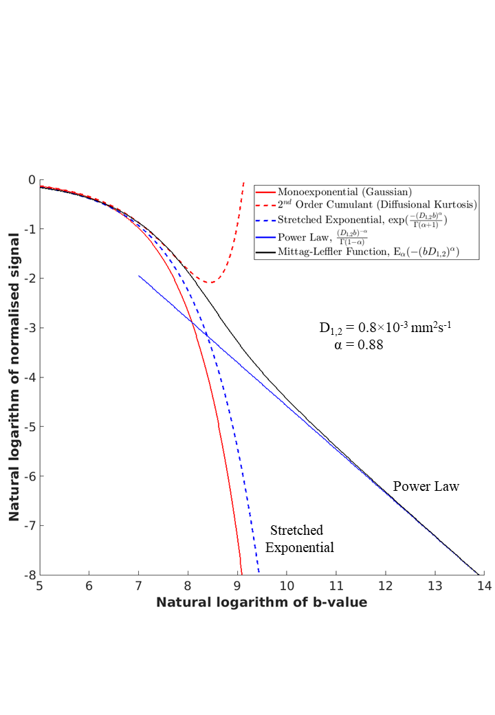
Ultra-high b-value diffusion MRI (dMRI) has potential to provide more accurate and sensitive detection of brain tissue microstructural characteristics^1,2. For moderate b-values ($$$1000{\leq}b{\leq}3000$$$ s mm^-2) the stretched exponential^3,4 and 2^nd order cumulant expansion^5,6 approximate dMRI signal decay in tissue. However, at high b-values ($$$8000{\leq}b{\leq}25000$$$ s mm^-2) a power law decay is observed^2,7, an effect predicted from approximating a diffusion signal restricted to regions near surface boundaries, the so-called “localisation regime”^8,9,10. In this study we investigate whether the quasi-diffusion model^11,12,13 describes the full dMRI decay curve to link these two extremes with a single function.

Quasi-Diffusion MRI (QDI) is derived from a special case of the Continuous Time Random Walk model of diffusion dynamics^11,12,13 and describes the diffusion decay curve as a stretched Mittag-Leffler function ($$$E_α$$$)^11,12,13,
$$E_{\alpha}(-(D_{1,2}b)^{\alpha})=\sum_{k=0}^{\infty}\frac{(-1)^{k}(D_{1,2} b)^{{\alpha}k}}{\Gamma({\alpha}k+1)}=\frac{S_{b}}{S_{0}},\;\;\;\;\;\;[1]
$$where $$$S$$$ is the signal, $$$\Gamma (x)$$$ the gamma function, $$$D_{1,2}$$$ the diffusion coefficient (in mm²s^-1) which describes the rate of decay, and $$$\alpha$$$ a fractional exponent describing the tail of the decay. Gaussian diffusion occurs when $$${\alpha}=1$$$, and non-Gaussian (i.e. restricted) when $$$0<\alpha{\leq}1$$$. The asymptotic properties of Eq.1 are,
$$E_{\alpha}(-(D_{1,2}b)^{\alpha})\sim\begin{cases}\mathrm{exp}[-\frac{b^{\alpha}}{\Gamma(\alpha+1)}],
\;\;\;\;\;\;\;\;\;\;\;\;\;\;b{\to}0,\;\;\;\;b{\ll}D_{1,2}\\\frac{b^{-\alpha}}{\Gamma(1-\alpha)}=\frac{\sin(\alpha\pi)}{\pi}\frac{\Gamma(\alpha)}{b^{\alpha}},\;\;\;\;b{\to}\infty,\;\;b{\gg}D_{1,2}\\\end{cases}\;\;\;\;\;\;[2]
$$and indicate QDI interpolates, via an inflection point (IP), between a stretched exponential at low b-values and a negative power law at high b-values¹².

Here we extend the application of QDI^11,13 by investigating the stability of $$$D_{1,2}$$$, $$$\alpha$$$ and signal IPs up to a maximum b-value of $$$15000$$$ s mm^-2. Furthermore, we investigate QDI accuracy in a clinically feasible dataset with fewer b-values.

Methods

Image Acquisition: An open source dataset of whole brain dMRI acquired from a healthy participant was used for analysis¹⁴. Acquisition parameters: $$$TE/TR=55/4000$$$ms, $$$\delta/\Delta=12/23$$$ms, 66 axial slices, 2mm isotropic resolution; six $$$b=0$$$ s mm^-2 images and eleven b-value shells $$$\{400,800,1200,2000,3000,4000,6000,8000,10000,12000,15000\}$$$ in $$$\{6,16,16,21,31,21,21,31,31,31,31,46\}$$$ diffusion gradient directions, respectively (acquisition time 20 minutes 8 seconds).

Image Analysis: dMRI were corrected for Gibbs ringing, motion and eddy current distortions, and Rician noise. The orientation averaged signal was used to estimate $$$D_{1,2}$$$ and $$$\alpha$$$ from,
$$\mathrm{ln}(\frac{S_{b}}{S_{0}})=\mathrm{ln}(E_{\alpha}(-(D_{1,2}b)^{\alpha})),\;\;\;\;\;\;[3]
$$using the trust-region-reflective algorithm¹⁵.

To assess the quasi-diffusion as a model of dMRI signal attenuation, $$$D_{1,2}$$$ and $$$\alpha$$$ were estimated between $$$b=0$$$ and maximum b-values in the range $$$1200{\leq}b{\leq}15000$$$ s mm^-2. b-value IPs were computed by differentiation of Eq.3. Mean and standard deviations of $$$D_{1,2}$$$, $$$\alpha$$$ and IPs were calculated in grey matter (GM) and white matter (WM).

To investigate whether $$$D_{1,2}$$$, $$$\alpha$$$ and IPs can be accurately estimated from dMRI acquired within clinically feasible time, measures were estimated from $$$b_{short}=\{0,1200,4000,15000\}$$$ s mm^-2 data (acquisition time 6 minutes 16 seconds). Two low b-values were chosen with one beyond expected tissue IPs. Bias (short acquisition measures minus full acquisition), uncertainty (standard deviation of differences) and Intraclass Correlation Coefficients (ICC) were calculated across all tissue voxels for $$$D_{1,2}$$$, $$$\alpha$$$ and IPs.

Results

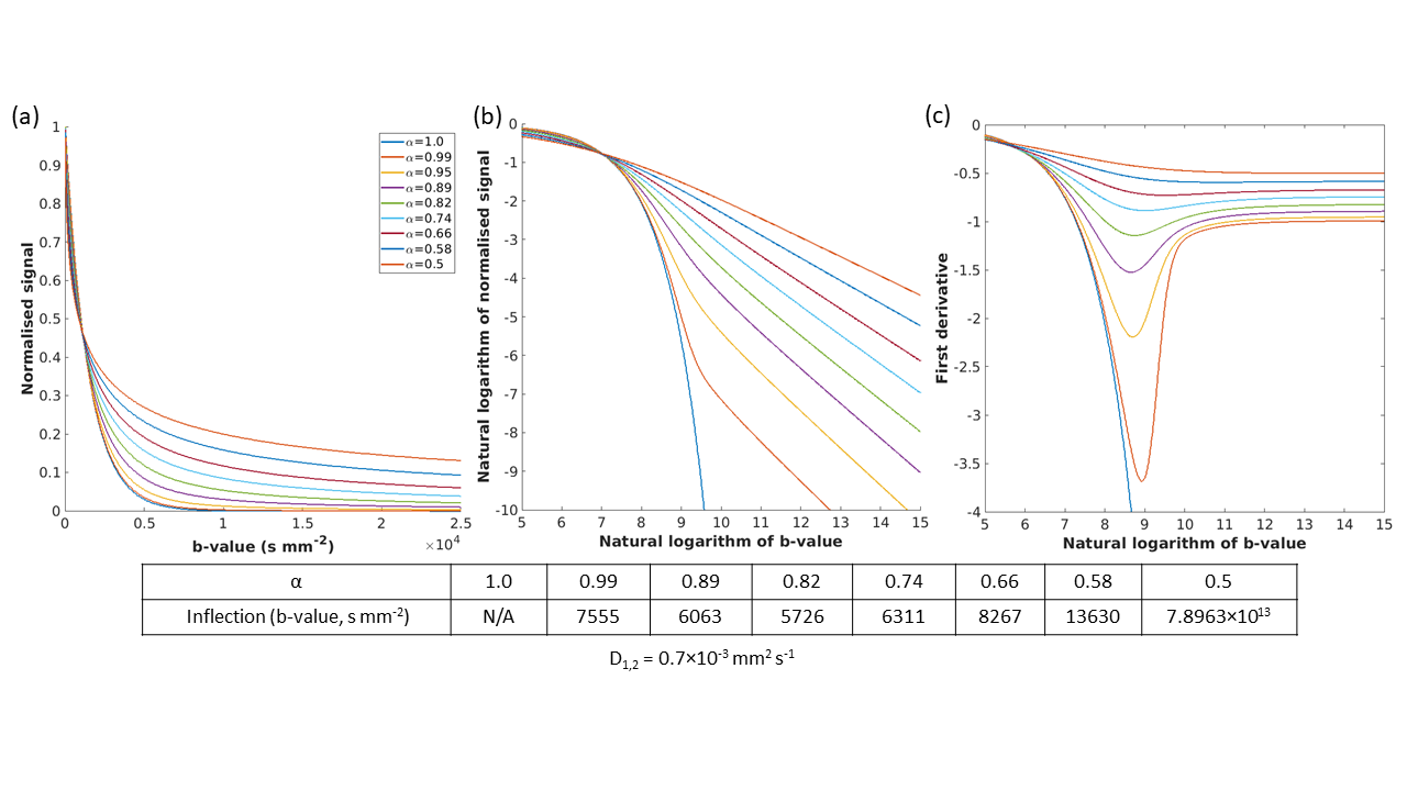
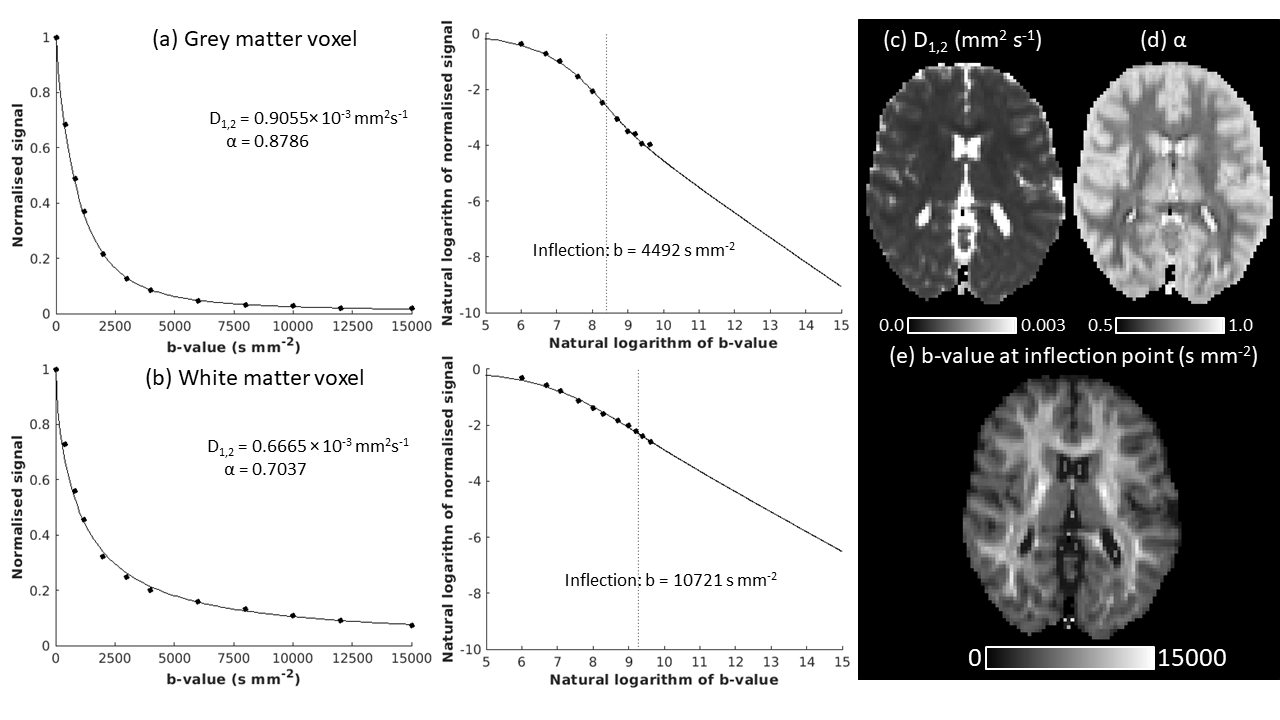
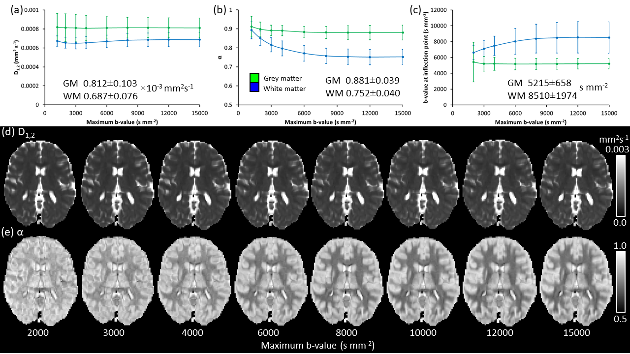
Fig.1 illustrates the extremal signal regimes of Eq.1, monoexponential, and kurtosis functions for a representative GM voxel. Fig.2 shows predicted quasi-diffusion signal attenuation for $$$D_{1,2}=0.7{\times}10^{-3}$$$ mm²s^-1 with $$$0.5{\leq}\alpha{\leq}1.0$$$ (Fig.2a) and demonstrates that each decay curve contains an inflection point (Fig.2b). In general, lower $$$\alpha$$$ leads to higher IPs. The first derivative in the logarithmic space (Fig.2c) indicates that after inflection the signal enters the localisation regime^8,9,10where the gradient tends to $$$-\alpha$$$.

Fig.3 shows excellent quasi-diffusion model fits to dMRI signal within representative GM (Fig.3a) and WM (Fig.3b) voxels for $$$0{\leq}b{\leq}15000$$$ s mm^-2, and illustrates signal inflection points. Maps of $$$D_{1,2}$$$ (Fig3c), $$$\alpha$$$ (Fig.3d) and IP (Fig3.e) demonstrate tissue specific values (Fig.4a to e) which tend to stable values as maximum b-value increases (see Fig.4). QDI parameters stabilise when maximum b-values approach or exceed the IP, which is at lower b-values in GM ($$$b{\geq}3000$$$) than WM ($$$b{\geq}8000$$$).

Fig.5 shows that $$$D_{1,2}$$$, $$$\alpha$$$ and IP are highly accurate and reproducible when fitted from $$$b_{short}$$$ compared to all data ($$$0{\leq}b{\leq}15000$$$ s mm^-2). ICCs were extremely high across brain tissue (Fig.5b). Measurement bias was small, $$${\approx}1\%$$$ of mean $$$D_{1,2}$$$, $$${\approx}0.4\%$$$ of mean $$$\alpha$$$, and $$${\approx}1.25\%$$$ of mean IP (Fig.5b).

Discussion and Conclusions

We have shown that the quasi-diffusion model fits to dMRI data across low and high b-value regimes via a single, parsimonious function with two independent parameters, $$$D_{1,2}$$$ and $$$\alpha$$$. Stable parameter estimates were identified upon increasing the maximum b-value, suggesting that quasi-diffusion is a valid model for dMRI signal in healthy brain tissue. Furthermore, QDI parameters computed from a 4 b-value acquisition are accurate and reproducible when compared to the full acquisition (12 b-values) indicating that QDI measurements may be accurately estimated from dMRI acquired in clinically feasible times.

Stable QDI parameters were observed when the maximum b-value approached signal IPs, indicating that the quasi-diffusion model can be used to identify the maximum b-values required at acquisition for accurate estimation of signal power law behaviour and the localisation regime. IP may provide a novel high SNR image contrast that is a composite of, $$$D_{1,2}$$$ and $$$\alpha$$$ with physical meaning. For directionally averaged signal in healthy tissue this corresponds to $$$b{\geq}8000$$$ s mm^-2. For reliable computation of power law anisotropy (i.e. anisotropy), or in tissue with low $$$\alpha$$$, we advocate acquisition of higher maximum b-values, and development of techniques that overcome effects of noise to enable reliable computation of $$$\alpha$$$ from low b-value ranges.

Acknowledgements

Imaging data used in this study was provided on request under a Creative Commons Attribution 4.0 International license. Afzali M (2022). Data for 'Cumulant Expansion with Localization: A new representation of the diffusion MRI signal'. Cardiff University. https://dx.doi.org/10.17035/d.2022.0215863820.

References

1. Afzali M, Pieciak T, Newm S, Garyfallidis E, Özarslan E, Cheng H, Jones DK, The sensitivity of diffusion MRI to microstructural properties and experimental factors. Journal of Neuroscience Methods 2021, 108951. https://doi.org/10.1016/j.jneumeth.2020.108951.

2. Veraart J, Fieremans E, Novikov DS. On the scaling behavior of water diffusion in human brain white matter. NeuroImage 2019, 185: 379-387.

3. Bennett KM, Schmainda KM, Bennett R, Rowe DB, Lu H, Hyde JS, Characterization of continuously distributed cortical water diffusion rates with a stretched-exponential model. Magn. Reson. Med. 2003, 50, 727–734.

4. Palombo M, Gabrielli A, De Santis S, Cametti C, Ruocco G, Capuani S, Spatio-temporal anomalous diffusion in heterogeneous media by nuclear magnetic resonance. J. Chem. Phys. 2011, 135, 034504, doi:10.1063/1.3610367.

5. Jensen JH, Helpern JA, Ramani A, Lu H, Kaczynski K, Diffusional Kurtosis Imaging: The quantification of non-Gaussian water diffusion by means of magnetic resonance imaging. Magn. Reson. Med. 2005, 53, 1432–1440.

6. Jensen JH, Helpern JA, MRI Quantification of non-Gaussian water diffusion by kurtosis analysis. NMR Biomed. 2010, 23, 698–710.

7. McKinnon ET, Jensen JH, Glenn GR, Helpern JA. Dependence on b-value of the direction-averaged diffusion-weighted imaging signal in brain. Magn Reson Imaging. 2017, 36:121-127.11.

8. de Swiet TM, Sen PN, Decay of nuclear magnetization by bounded diffusion in a constant field gradient. J. Chem. Phys. 1994, 100, 5597–5604.

9. Moutal N, Demberg K, Grebenkov DS, Kuder TA, Localization regime in diffusion NMR: Theory and experiments, Journal of Magnetic Resonance 2019, 305: 162-174.

10. Moutal N, Grebenkov, DS, The localization regime in a nutshell. Journal of Magnetic Resonance 2020, 320, 106836. doi: 10.1016/j.jmr.2020.106836.

11. Barrick TR, Spilling CA, Ingo C, Madigan J, Isaacs JD, Rich P, Jones TL, Magin RL, Hall MG, Howe FA, Quasi-Diffusion Magnetic Resonance Imaging (QDI): A fast, high b-Value diffusion imaging technique. NeuroImage 2020, 211, 116606.

12. Barrick TR, Spilling CA, Hall MG, Howe FA, The mathematics of quasi-diffusion magnetic resonance imaging. Mathematics 2021, 9(15), 1763. doi:10.3390/math9151763.

13. Spilling, C.A., Howe FA, Barrick TR, Optimization of quasi-diffusion magnetic resonance imaging for quantitative accuracy and time-efficient acquisition. Magn. Reson. Med. 2022, 88, 2532-2547.

14. Afzali M, Pieciak T, Jones DK, Schneider JE, Özarslan E, Cumulant expansion with localization: A new representation of the diffusion MRI signal. Front Neuroimaging 2022, https://doi.org/10.3389/fnimg.2022.958680.

15. lsqcurvefit, Matlab, Mathworks, Inc, https://uk.mathworks.com/help/optim/ug/lsqcurvefit.html.

Figures

Figure 1: Predicted signal attenuation for the quasi-diffusion model. The stretched Mittag-Leffler function is illustrated and its transition between a stretched exponential at low b-values and a negative power law at high b-values. The transition is marked by an inflection point. Predicted signal attenuation is shown for D_1,2=0.8×10^-3 mm²s^-1 and α = 0.88. Gaussian (monoexponential) and 2^nd order cumulant (Diffusional Kurtosis) approximations are also shown.

Figure 2: Predicted signal attenuation for the quasi-diffusion model when D_1,2=0.7×10^-3 mm²s^-1 and 0.5 ≤ α ≤1. Graph (a) shows the normalised signal attenuation for the family of curves. Graph (b) shows signal attenuation on a log log plot (using the natural logarithm). Graph (c) shows the first derivative of the log log plot. b-value inflection points (IP) are identified by the minimum of this gradient. At high b-values the gradient tends to -α. The table indicates IP for each α.

Figure 3: Signal attenuation for representative (a) grey matter, and (b) white matter voxels are shown with axial slices of (c) D_1,2, (d) α and (e) IP. Signal attenuation is shown for normalised signal (left graphs), and on a log log plot (right graphs). Fitted D_1,2 and α values are shown with the location of the IP.

Figure 4: Graphs of computed (a) D_1,2, (b) α and (c) IP shown with increasing maximum b-value for grey and white matter regions of interest. Mean and standard deviation of D_1,2, α and IP are presented within grey matter (coloured green) and white matter (coloured blue). Axial slices for (d) D_1,2 and (e) α computed over different maximum b-values are also shown. Tissue values computed for 0 ≤ b ≤ 15000 s mm^-2 are shown as text on graphs (mean±standard deviation).

Figure 5: Comparison of D_1,2, α and IP calculated from the full acquisition (12 b-values, 0 ≤ b ≤ 15000 s mm^-2) and an example subset of the data (4 b-values, b_short = {0,1200,4000,15000} s mm^-2). Maps of (a) D_1,2, (b) α and (c) IP are shown for the full acquisition (left column), and data subset (middle column). Graphs (right column) show scatter plots of D_1,2, α and IP computed for the data subset against the full acquisition. Intraclass correlation coefficients (ICC) and bias±uncertainty are shown as text on graphs.

Proc. Intl. Soc. Mag. Reson. Med. 31 (2023)

0759

DOI: https://doi.org/10.58530/2023/0759