Synopsis

Keywords: Flow, Velocity & Flow, CFD

Aortic hemodynamic quantifications are vital for patient management. While 4D Flow MRI provides comprehensive aortic hemodynamics, it is hampered by long-acquisition times and cumbersome pre-processing. In this study, we developed an AI for the prediction of systolic 3D blood flow velocity vector fields with 3D aortic geometry as the only input. We performed testing on 248 BAV and 104 TAV datasets, using the systolic velocity vector fields from the 4D flow MRI as the ground-truth. Generally, we saw very strong agreement between the AI and the 4D flow and resilience to geometric changes (volume, dimension) in the input segmentation.

Introduction

Quantification of aortic flow is vital for patient management in a number of aortic and heart valve diseases. While 4D Flow MRI provides a comprehensive assessment of aortic hemodynamics, it requires long acquisition times, cumbersome pre-processing, and is not widely available. In contrast, Computational Fluid Dynamics (CFD) is capable of simulating 3D blood flow dynamics from aortic geometry. However, it is hampered by requiring user-defined boundary conditions, long computation times, and patient-specific in-flow and pressure conditions [1]. Recently, artificial intelligence (AI) has shown success in image-to-image translation [2]. Previously, we introduced the concept of AI-derived aortic hemodynamics through a cycleGAN to predict aortic systolic absolute velocities [3]. Here, we expanded on this work for the prediction of systolic 3D blood flow velocity vector fields with 3D aortic geometry as the only input. This study expanded the training and testing data for both bicuspid aortic valve (BAV) and tricuspid aortic valve (TAV) as well as systematically investigated the resilience of the AI network to changes in the input 3D aortic geometry.

Methods

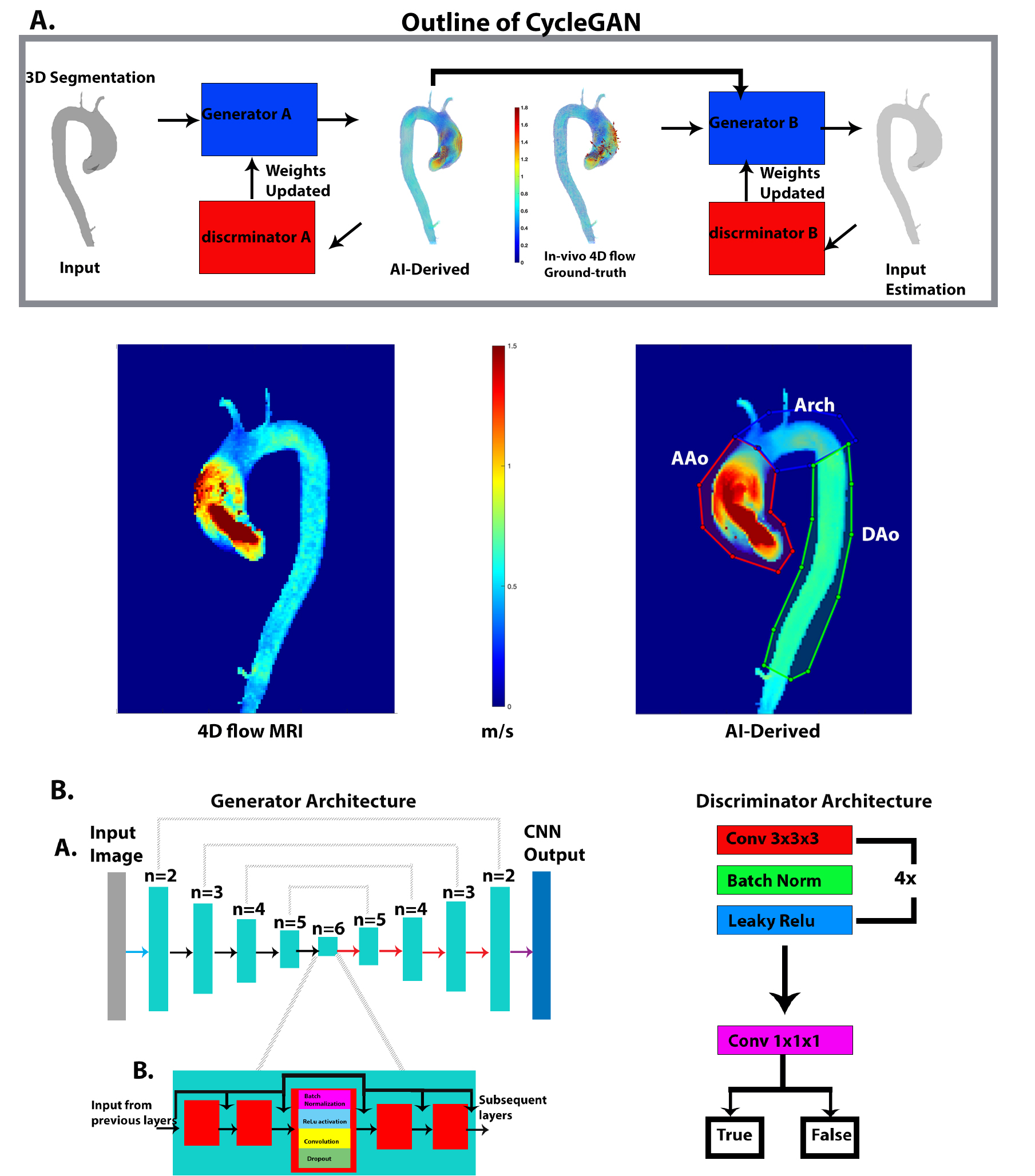
This study used a total of aortic 4D flow MRI data in N=1765 patients (1242 BAV, median age:42 years; 523 TAV, median age:45 years), acquired on either 1.5T or 3T MRI systems (Siemens). All 4D flow MRI data were acquired with 3D coverage of the thoracic aorta and the following sequence parameters: spatial res=1.2-5.0mm3, venc=150-500cm/s, temp res=32.8-44.8ms. For all 1765 subjects, a 3D segmentation of the thoracic aorta (used as CycleGAN input) was generated from the 4D flow and used to extract the systolic 3D blood flow velocity vector field inside the aorta (ground-truth data). Two separate CycleGANs were trained: one for BAV and another for TAV. For AI training, we used 994 BAV and 419 TAV datasets, while AI testing was performed on 248 BAV and 104 TAV (80%/20% split). The CycleGAN was composed of two generators and two discriminators [2] (Figure 1A). The generators used a 3D hybrid Densenet/Unet [4, 5] (Figure 1B). Discriminators were based on 5 convolution layers with 4x4 kernel size (Figure 1B). For the loss function, we incorporated the original loss functions of the cycleGAN and a SSIM loss $$$(1-SSIM)$$$. Additionally to enforce divergence-free conditions of incompressible flow for the AI-estimation, we added a velocity gradient loss [6] as:

$$GradientLoss=\frac{1}{X*Y*Z}\sum_{x=1}^X\sum_{y=1}^Y\sum_{z=1}^Z((\frac{dV_x^{gt}}{dx}-\frac{dV_x^{ai}}{dx})^2+(\frac{dV_y^{gt}}{dy}-\frac{dV_y^{ai}}{dy})^2+(\frac{dV_z^{gt}}{dz}-\frac{dV_z^{ai}}{dz})^2)$$

Where X, Y, Z are height, width, and depth, and gt is the ground-truth 4D flow.

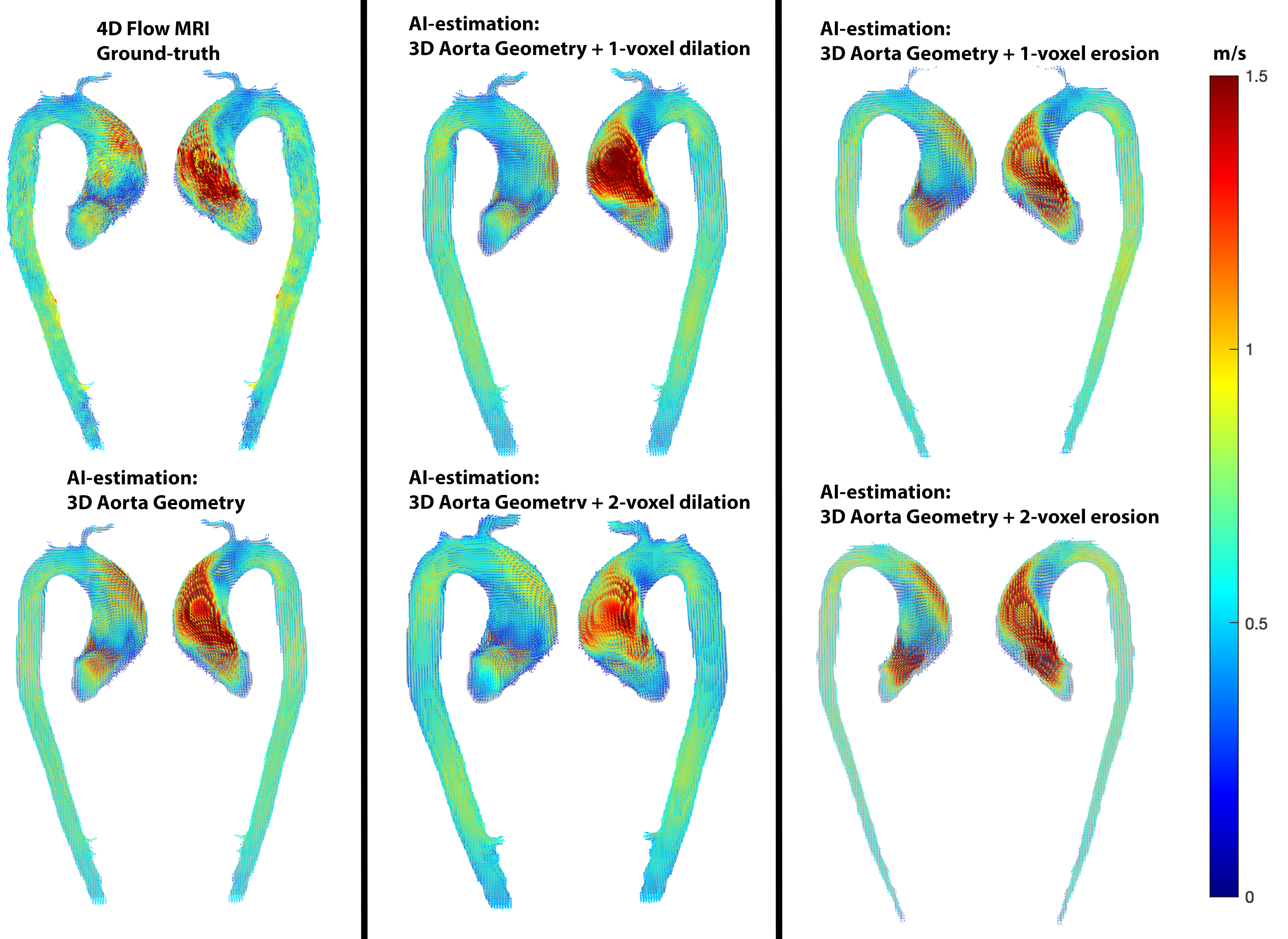
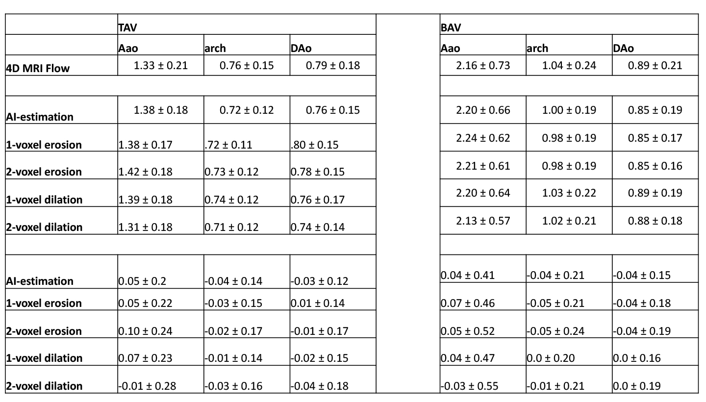
For each testing datasets, 1 or 2-voxel erosion and dilation were performed on the input 3D segmentation in order to assess the robustness of the AI network for predicting the systolic 3D velocity vector field inside the aorta despite changes in the aortic dimensions and total volume. Region of interest analysis was used to quantify peak velocities (top 5%) in the ascending (AAo), arch, and descending aorta (DAo) (Figure 1). Comparisons were performed using 3D vector field plots, and voxel-by-voxel (in the unmodified 3D geometry) and regional peak velocity Bland-Altman analysis across all datasets.

Results

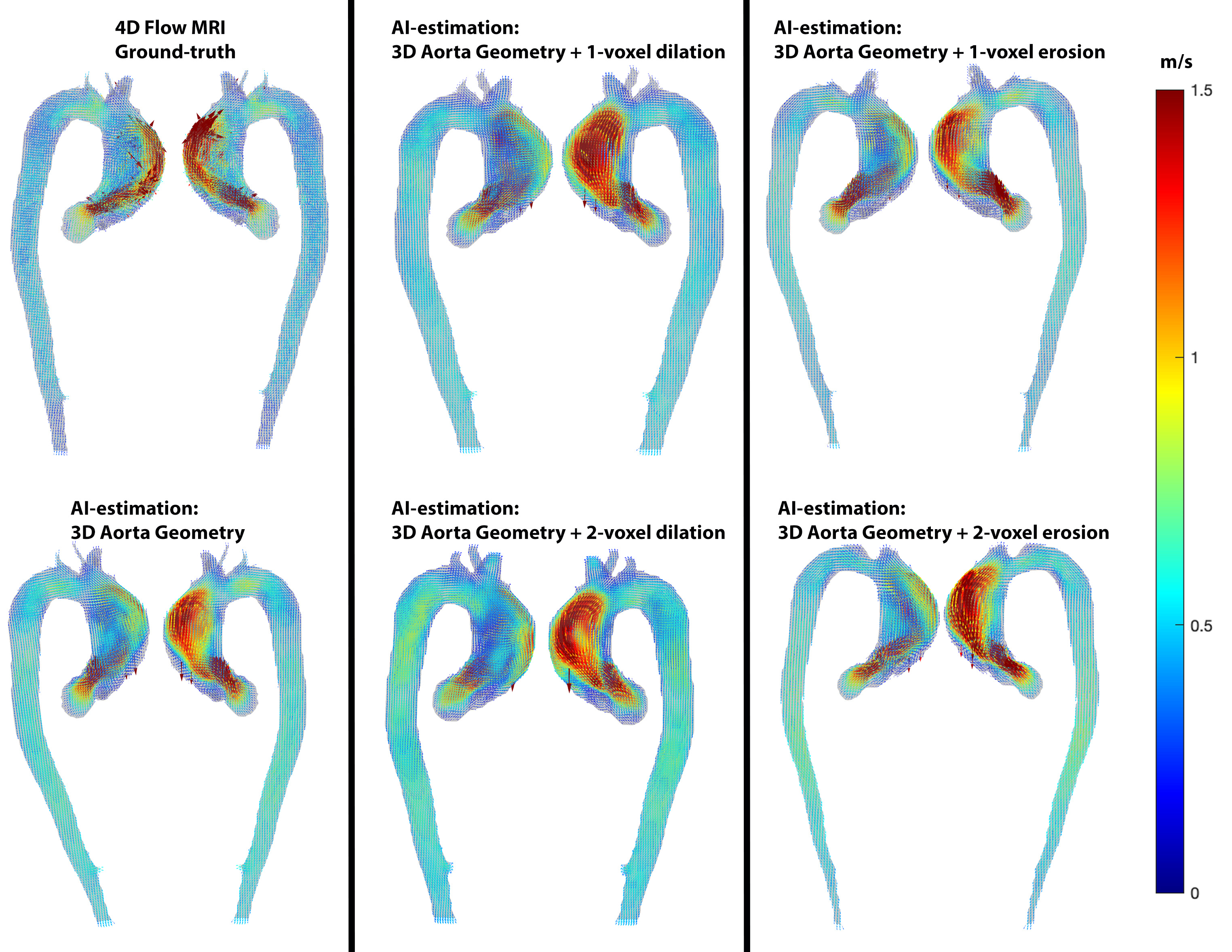
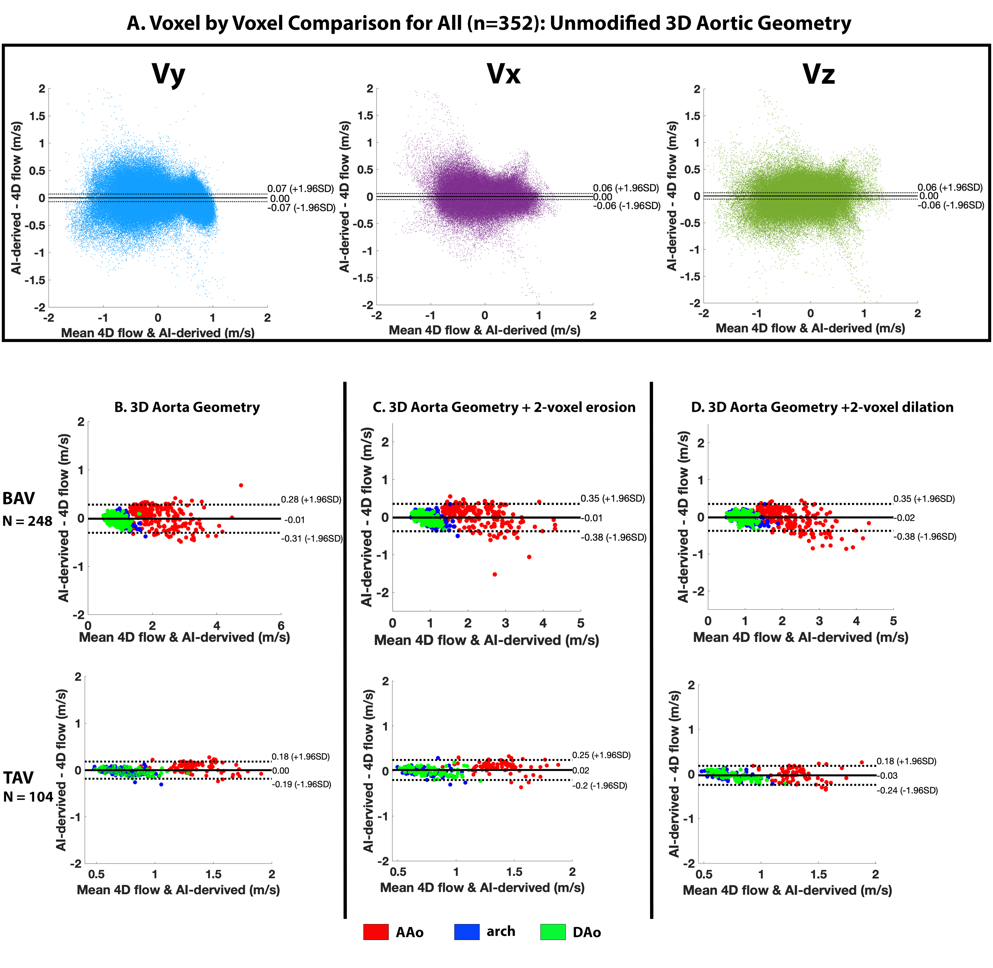
AI computation time was 0.15±0.11s, while total training time was 3600 min. Figure 2 illustrates AI performance for one of the best and Figure 3 for the worst cases. Figure 2 shows the ground-truth 4D flow and AI-estimated systolic 3D blood flow velocities across all variations of the input segmentation (3D geometry). All AI derived aortic 3D velocity vector fields showed similar velocity patterns across the aorta — such as a marked valve jet flow pattern along the left anterior wall of the AAo. Figure 3 shows one of the worst cases in which the AI-estimated systolic 3D blood flow velocities resulted in an incorrect jet-flow pattern in AAo traveling along the opposite side of the AAo. Nonetheless, the AI reproduced consistent velocity vector field estimations independent of the changes (erosion and dilation) of the 3D input geometry. Bland-Altman analysis comparing AI-estimated vs. 4D flow voxel-by-voxel (Vx,Vy,Vz) and regional aortic peak velocities are shown in Figure 4 and summarized in Table 1 (average peak velocity and bias and limits of agreements across all of the datasets). For voxel-by-voxel comparisons, the AI showed low bias and excellent limits of agreements (±0.06-0.07m/s) across all datasets (Figure 4A). For the non-modified 3D aortic geometry peak velocities, the AI showed a low bias (AAo: 0.04-0.05 m/s, arch: -0.04m/s, DAo: -0.04- -0.03m/s) and narrow limits of agreement: AAo: ±0.20-0.41m/s, arch: ±0.14-0.21m/s, DAo: ±0.12-0.15m/s across the BAV and TAV datasets (Figure. 4B). For the 1-voxel erosion and dilation of the 3D aortic geometry, the AI performance was undisturbed with only mildly increased bias (AAo: 0.04-0.07m/s, arch: -0.05-0.0m/s, DAo: -0.04-0.01m/s) and small limits of agreements: AAo: ±0.22-0.47m/s, arch: ±0.14-0.21m/s, DAo: ±0.12-0.18m/s. Finally, for the two voxel-erosion and dilation of the 3D aortic geometry, greater discrepancies were observed with increased bias compared to the ground-truth 4D flow data (AAo: -0.03-0.1m/s, arch: -0.05- -0.01m/s, DAo: -0.04-0.0m/s) and moderate limits of agreements: AAo: ±0.24-0.55m/s, arch: ±0.16-0.24m/s, DAo: ±0.17-0.19m/s (Figure 4C,D).

Conclusion

AI-derived systolic velocity vector fields showed strong agreement to the 4D flow MRI and was resilient to geometric changes (volume, dimension) in the input segmentation. Future direction is to expand this work for CT-derived 3D aortic geometry and explore AI-based WSS estimations.

Acknowledgements

No acknowledgement found.