0475
Evaluation of Deep Learning Models for Processing Lactate-Edited MR Spectroscopic Imaging in Patients with Glioma
Sana Vaziri1, Adam W Autry1, Marisa Lafontaine1, Janine Lupo1, Susan Chang2, and Yan Li1
1Radiology and Biomedical Imaging, University of California, San Francisco, San Francisco, CA, United States, 2Neurological Surgery, University of California, San Francisco, San Francisco, CA, United States
1Radiology and Biomedical Imaging, University of California, San Francisco, San Francisco, CA, United States, 2Neurological Surgery, University of California, San Francisco, San Francisco, CA, United States
Synopsis
Keywords: Data Processing, Spectroscopy
The use of deep learning models for frequency and phase correction of spectral data was evaluated to reduce processing time of 3D MRSI datasets acquired from patients with glioma. Models for frequency and phase offset estimation were trained for data prior to coil-combination. Separate models for baseline removal of coil-combined data were similarly trained and evaluated. The voxel-wise peaks for spectra processed using the standard approach were evaluated and compared to the spectra processed using the proposed deep learning approach. Compared to standard processing, deep learning processing produced spectra with comparable SNR and linewidths in a shorter processing time.Introduction
1H MR spectroscopic imaging (MRSI) is a powerful noninvasive technique that allows for the measurements of brain metabolites, such as N-acetyl-aspartate (NAA), choline-containing compound (Cho), and creatine (Cr). Lactate-editing allows the separation of lactate peaks1, a biomarker for anaerobic metabolism, from lipid signals, which indicate necrosis or aliasing from subcutaneous tissue. Although previous studies have demonstrated the importance of using 3D lactate-edited MRSI for evaluating patients with glioma2, one of the challenges for its clinical translation is long and complicated data processing. Artifacts caused by subject motion, lipid suppression, and water peak removal may result in frequency and phase offsets in the resulting spectra. While the use of phased-array receive coils can improve SNR3, the frequency/phase variations among channels may cause broadened metabolite peaks, reduced SNR, and distorted baseline after coil combination. Standard MRSI processing procedures include voxel-wise frequency and phase corrections, coil combination, and baseline removal prior to quantification4,5,6. Recently, a deep learning (DL) approach for spectral frequency and phase corrections was introduced for offset estimation of individual transients before averaging7, greatly reducing processing time. In this work, we evaluated the use of DL models for voxel-wise frequency/phase correction and baseline removal for 3D lactate-edited MRSI datasets acquired from patients with glioma.Methods
MRI and MRSI Data: A total of 37 datasets (35 training/validation, 2 test) were acquired from patients with glioma using an 8-channel phased-array head coil on 3T MR scanners (GE Healthcare, Waukesha, WI). A proton density-weighted gradient echo images for obtaining estimates of coil sensitivities and 3D lactate-edited MRSI datasets (TE=144ms, TR=1300ms, 1cm isotropic spatial resolution, matrix size = 16-18 x 16-18 x 16, flyback in the SI direction, 2 cycles (Edit-On/Edit-Off), total acquisition time ~10 min) were added to the standard brain tumor protocol.Processing of spectral data and generation of DL training data: The spectral data were preprocessed with reordering to the rectilinear grid, apodization using a 4Hz Lorentzian filter, zero-filling to 1024 points, and Fourier transformation to spectral domain1. Training data for DL models were created using standard processing (ST)5,6, that utilized residual water peaks removed from Edit-OFF cycle spectra by HSVD filter8 for frequency/phase estimations. The phase/frequency-corrected spectra were then combined using an in-house software weighting with coil sensitivities9. ST included an additional round of frequency/phase estimation on the combined spectra3, not performed in DL processing. The ST estimated combined-spectra baseline was used as the training output for the DL model. The heights of Cho, Cr, and NAA were then estimated from baseline removed spectra with prior knowledge of peak locations.
DL network architecture and processing: DL networks are shown in Figure 1 and the DL-based processing workflow is summarized in Figure 2. Magnitude spectra were used as input to the frequency estimation model and real-valued spectra were used for the phase estimation model7. Baseline estimation models (Figure 1b) were trained on coil-combined data. Voxels within the excitation regions were aggregated from 35 datasets and used to train the DL models (Figure 3). All models were trained on a custom workstation with AMD 3900X 12-core CPU with a Nvidia Titan X GPU with Python 3.8 and Tensorflow 2.2.
Spectral analysis: ST and DL processing was performed on the remaining 2 datasets not used in training. Root-mean-square errors (RMSE) comparing DL to ST estimated offsets were calculated. Metabolite (NAA, Cho, Cr) SNR and linewidths5 were estimated from both processing methods. Pearson’s correlation coefficients were calculated to assess voxel-wise correlations between the two methods.
Results
Training/prediction times for DL models are summarized in Figure 3. Frequency/phase prediction times for one 8 channel 3D dataset (18x18x16x8-channel = 41,472 spectra) were <3 minutes each. Baseline predictions for one 3D dataset were <1 minute (18x18x16 = 5,184 coil-combined spectra). DL models successfully estimated frequency and phase in the test datasets for individual channel data (RMSE=7.9 for frequency. RMSE for phase was not included as the measurements are in degrees). An example of final ST and DL processed spectra are displayed in Figure 4b, showing agreement between the two methods. A comparison of the spectral analysis of the ST and DL processed spectra are shown in Figure 5. The SNR and linewidths values for all metabolites were correlated (SNR: R>0.9 all metabolites, linewidth: R>0.6 all metabolites) indicating the data processed with DL agreed well with ST.Discussion and conclusion
Post-processing of spectral data can be time-consuming and complex. Recently introduced DL-based methods for frequency/phase correction both reduce processing time and simplify overall workflow. In this work, the use of a DL model for frequency and phase correction applied prior to coil combination was evaluated on patient data. We also created a DL model for baseline estimation, which is an important step before quantifying long TE MRSI. Although the ST processing pipeline included an additional frequency/phase correction step following coil combination, DL metabolite peak SNR and linewidths were similar to ST. Further improvements to the DL processing may be seen after a second such correction prior to baseline removal (see highlighted voxels in Figure 4b). Future work will include an additional model to estimate and remove the water peak along with the evaluation of more complex models for frequency and phase correction.Acknowledgements
This project was supported by NIH T32 CA151022, R01 CA262630, P01 CA118816, P41EB013598, P50 CA097257, Department of Defense W81XWH2010292, and the Glioblastoma Precision Medicine Program.References
- Park, Ilwoo, et al. "Implementation of 3 T lactate-edited 3D 1H MR spectroscopic imaging with flyback echo-planar readout for gliomas patients." Annals of biomedical engineering 39.1 (2011): 193-204.
- Nelson, Sarah J., et al. "Serial analysis of 3D H-1 MRSI for patients with newly diagnosed GBM treated with combination therapy that includes bevacizumab." Journal of neuro-oncology 130.1 (2016): 171-179.
- Vareth, Maryam, et al. "A comparison of coil combination strategies in 3D multi‐channel MRSI reconstruction for patients with brain tumors." NMR in Biomedicine 31.11 (2018): e3929
- Nelson, Sarah J., et al. "Association of early changes in 1H MRSI parameters with survival for patients with newly diagnosed glioblastoma receiving a multimodality treatment regimen." Neuro-oncology 19.3 (2017): 430-439.
- Nelson, Sarah J. "Analysis of volume MRI and MR spectroscopic imaging data for the evaluation of patients with brain tumors." Magnetic Resonance in Medicine: An Official Journal of the International Society for Magnetic Resonance in Medicine 46.2 (2001): 228-239.
- Li, Yan, et al. "Considerations in applying 3D PRESS H-1 brain MRSI with an eight-channel phased-array coil at 3 T." Magnetic Resonance Imaging 24.10 (2006): 1295-1302.
- Tapper, Sofie, et al. "Frequency and phase correction of J‐difference edited MR spectra using deep learning." Magnetic resonance in medicine 85.4 (2021): 1755-1765.
- Coron, Alain, et al. "The filtering approach to solvent peak suppression in MRS: a critical review." Journal of Magnetic Resonance 152.1 (2001): 26-40.
- Crane, Jason C., Marram P. Olson, and Sarah J. Nelson. "SIVIC: open-source, standards-based software for DICOM MR spectroscopy workflows." International journal of biomedical imaging 2013 (2013).
Figures
Figure 1: DL network architectures. (a) Phase and frequency networks7 consisted of 1 input layer, 2 fully connected hidden layers, and a single fully connected output layer. (b) The baseline estimation model consists of 2 fully connected hidden layers and a single fully connected output layer. The model was trained twice: once using the real component of the standard processing baseline and once using the imaginary component of the standard processing baseline estimate.
Figure 2: DL processing workflow. Individual channel edit-OFF cycle data (with the water peak included) are used as input to the DL frequency/phase models for prediction of offsets, which are then applied to the edit-OFF (water peak removed using HSVD) and edit-ON data. Following DL frequency/phase corrections, individual coil data are combined. The real and imaginary components of the baseline are then estimated and subtracted to produce the final DL processed spectra. This process is done for all voxels in a 3D dataset.
Figure 3: DL model details and timings. All models were trained utilizing Python 3.8 and Tensorflow 2.2 (batch size=64, 500 epochs). The frequency/phase estimation models were trained on voxels within the excitation region of 35 training datasets (110,246 channel-wise spectra). The baseline estimation models were trained on 13,968 channel-combined spectra. Training times are shown as an average of 10 runs. Prediction times are shown for a single complete e 8x18x18x16 dataset (41,472 individual channel spectra and 5,184 coil-combined spectra), average of 10 runs.
Figure 4: Standard processing vs DL processing. (a) Frequency/phase estimates from DL compared to ST from various voxels within the PRESS box for a single 3D lactate-edited MRSI dataset. Spectra from a single channel are shown for the edit-OFF and edit-ON cycles with ST corrected spectra (white) and DL corrected spectra (blue). (b) Final ST (white) and DL (blue) coil-combined spectra are shown (middle) for the slice displayed (left). Two sample voxels are highlighted on the right.
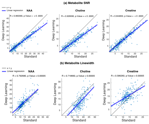
Figure 5: Standard vs Deep learning Spectral Analysis. Voxel-wise comparisons of metabolite SNR (a) and linewidth (b) are shown for the dataset from Figure 4. The blue line indicates the linear regression line (Pearson’s R and p-value displayed).
DOI: https://doi.org/10.58530/2023/0475