0352
Motion Correction in Brain MRI using Deep Image Prior
Jongyeon Lee1, Wonil Lee1, and HyunWook Park1
1Korea Advanced Institute of Science and Technology, Daejeon, Korea, Republic of
1Korea Advanced Institute of Science and Technology, Daejeon, Korea, Republic of
Synopsis
Keywords: Motion Correction, Motion Correction, Brain Motion Correction
Motion correction in MRI has been successful with deep learning techniques to reduce motion artifacts. However, these methods were based on supervised learning, which have required a large dataset to train neural networks. To overcome this issue, we propose a new technique to correct motion artifacts without any training dataset, which optimizes a neural network only with a single motion-corrupted image. We adopt Deep Image Prior framework to capture image priors from a convolutional neural network using motion simulation based on MR physics. Using the deep image prior, our method finely reduces motion artifacts without any dataset.Introduction
Motion correction techniques have been studied to reduce motion artifacts, which are caused by movements during scan. Conventional techniques usually require extra motion information for motion estimation and have a cost of a prolonged scan time1. Deep learning algorithms have been recently introduced to correct the artifacts in MR images without motion information or estimation2.Most of the deep learning methods are supervised-learning approaches that train convolutional neural networks (CNNs) from realistic data priors, hence require a large training dataset3. However, these methods rely on a training dataset. Recent motion correction methods with deep learning utilize motion simulation to overcome the training data shortage issue2. Instead of depending on the training dataset, an optimization scheme to capture image priors by the network structure, which is called Deep Image Prior (DIP), has been recently studied to restore images from given degraded images without ground truth images3. DIP only relies on optimizing an untrained CNN to produce naturally-looking images, including MR images4. This approach does not require a training dataset and a training process, but only needs a single degraded image to be corrected.
In this study, we propose a new motion correction technique using DIP to correct motion artifacts in MRI, especially for brain, without any training dataset. Our proposed framework consists of a CNN that captures structural priors, a spatial transformer network5 (STN) that transforms a CNN output image, and a motion simulation model that takes transformed images to synthesize a motion-simulated image. This framework enables motion correction only with a single motion-corrupted image by optimizing the randomly initialized networks. An overview of our proposed framework is illustrated in Figure 1.
Methods
DIP takes a fixed random noise, $$$\mathbf{z}$$$, with a uniform distribution from 0 to 1 as an input. Then, DIP optimizes a randomly initialized CNN, $$$f_\theta$$$, and STN, $$$g_\psi$$$, to generate an output image $$$\mathbf{x}=f_\theta(\mathbf{z})$$$ and its rigidly transformed images $$$\{{\mathbf{x}^{\text{T}_k}}\}^N_{k=1}$$$ where $$$N$$$ is the number of imaging segments. The $$$k$$$-th image $$$\mathbf{x}^{\text{T}_k}$$$ is consistent with a motion state at segment $$$k$$$. To prevent ill-posed problem, the spatial transformation is not applied to one of $$$N$$$-images and this image $$$\mathbf{x}^{\text{T}_\text{R}}=\mathbf{x}$$$ is set to be the reference image for transformation. In this study, the number of segments (equal to the turbo factor in turbo spin-echo sequence) $$$N$$$ is 16 and the reference image $$$\mathbf{x}^{\text{T}_\text{R}}$$$ is set with $$$\text{T}_\text{R}=\text{T}_{N/2}=\text{T}_8$$$.Taking the transformed images with corresponding k-space masks $$$\{{m^{k}}\}^N_{k=1}$$$, which are decided based on MR sequence, as input, the motion simulation model $$$\mathbf{M}(\cdot)$$$ synthesizes a motion-simulated image
$$\hat{\mathbf{y}}=\mathbf{M}(\{{\mathbf{x}^{\text{T}_k},m^k}\}^N_{k=1})=\mathcal{F}^{-1} \left({\sum_{k=1}^N{\mathcal{F}{(\mathbf{\mathbf{x}^{\text{T}_k}})\odot{m^k}}}}\right),$$
where $$$\mathcal{F}(\cdot)$$$ and $$$\mathcal{F}^{-1}(\cdot)$$$ is the forward and inverse Fourier transform operators, respectively, and $$$\odot$$$ is the element-wise product operator. The motion simulation model is visualized in Figure 2. The optimization process is formalized as
$$\theta^*=\arg\min_\theta \mathcal{L}(\mathbf{y},\hat{\mathbf{y}}),$$
where $$$\mathcal{L}(\cdot)$$$ is the loss function to be minimized. The output of the optimized CNN $$$\mathbf{x}^*=f_\theta^*(\mathbf{z})$$$ then becomes a motion-free image and the output of the optimized STN $$$\{{\mathbf{x}^{\text{T}_k}}\}^N_{k=1}=g_{\psi^*}(\mathbf{x}^*)$$$ then become spatially transformed motion-free images. The loss function $$$\mathcal{L}(\cdot)$$$ is formulated with SSIM loss and the mean absolute error (MAE) as
$$\mathcal{L}({\mathbf{y},\hat{\mathbf{y}}})=-\log\left(\text{SSIM}({\mathbf{y},\hat{\mathbf{y}})+1}\over{2}\right)+\lambda_{\text{MAE}}|{\mathbf{y},\hat{\mathbf{y}}}|,$$
where $$$\lambda_{\text{MAE}}=0.001$$$ in this study.
CNN consists of $$$U$$$-blocks of a convolutional layer, an instance normalization, leaky ReLU, and a bilinear up-sampling layer, and a last convolutional layer that produces an output image. In this study, as we set the dimension of the input noise as 16⨯16 and $$$U$$$ of 16, the number of up-sampling to have a 256⨯256 image as the output of CNN. Our STN is modified to have $$$N$$$-multi-layer perceptrons (MLPs) from the original STN, which has a single MLP, in order to produce $$$N$$$-motion parameters to generate $$$N$$$-transformed images. These networks are depicted in Figure 3.
All of the processes are performed with 32-coil channel data while the input noise has 1 channel and the output images has 64 channels (32 for real and 32 for imaginary).
MR brain images were acquired with a T2w turbo spin-echo sequence. Obtained from 3D T2w data, 2D MR data are used to simulate in-plane motion artifacts. Then, we randomly simulate motions for k-space segments to test our proposed method. Test data are 224 slices from 14 subjects, which were acquired at 3T scanner (Verio, Siemens). All MRI imaging were approved by the KAIST Institutional Review Board (IRB), and all participants signed the informed consent forms.
Experiments and Results
Sum-of-square corrected images $$$\hat{\mathbf{y}}_\text{SOS}=({\sum^{64}_{i=1}{\hat{\mathbf{y}}_i^2}})^{1/2}$$$ are used for visualization and evaluation. Random motions with various numbers of motions (from 1 to 4) are applied to generate motion-simulated images. Only in-plane motion artifacts are considered and simulated.As shown in Table 1, our proposed method successfully corrects motion artifacts without any training dataset for any motions tested. Figure 4 gives some example images with three motions that greatly reconstruct motion-free images and show STNs work properly.
Discussion and Conclusion
Although this method does not require training, optimization is time-consuming because a few thousands of iterations are needed to correct a single corrupted image. The optimization sometimes fails at an early stage so that re-optimization is unavoidable.We propose the motion correction method using DIP without training dataset and the proposed method successfully reduces motion artifacts from a single corrupted image.
Acknowledgements
This work was supported by the Korea Medical Device Development Fund grant funded by the Korea government (the Ministry of Science and ICT, the Ministry of Trade, Industry and Energy, the Ministry of Health & Welfare, the Ministry of Food and Drug Safety) (Project Number: 1711138003, KMDF-RnD KMDF_PR_20200901_0041-2021-02).References
- Zaitsev M, Maclaren J, Herbst M. Motion artifacts in MRI: A complex problem with many partial solutions. Journal of Magnetic Resonance Imaging. 2015;42(4):887-901.
- Lee J, Kim B, Park H. MC2‐Net: motion correction network for multi‐contrast brain MRI. Magnetic Resonance in Medicine. 2021;86(2):1077-1092.
- Ulyanov D, Vedaldi A, Lempitsky V. Deep image prior. In Proceedings of the IEEE Conference on Computer Vision and Pattern Recognition. 2018: 9446-9454.
- Yoo J, Jin KH, Gupta H, Yerly J, Stuber M, Unser M. Time-dependent deep image prior for dynamic MRI. IEEE Transactions on Medical Imaging. 2021: 40(12), 3337-3348.
- Jaderberg M, Simonyan K, Zisserman A. Spatial transformer networks. Advances in neural information processing systems. 2015: 28.
Figures
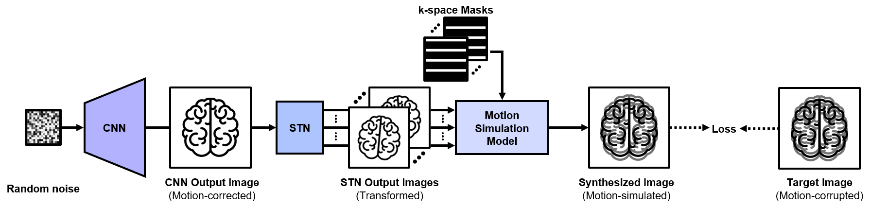
Figure 1. An
overview of the proposed framework. The fixed random noise is taken as CNN
input and CNN output becomes STN input. STN produces $$$N$$$-transformed
images to synthesize motion-simulated image with k-space masks. These networks
are optimized to minimize a loss function between the synthesized image and a
target image.
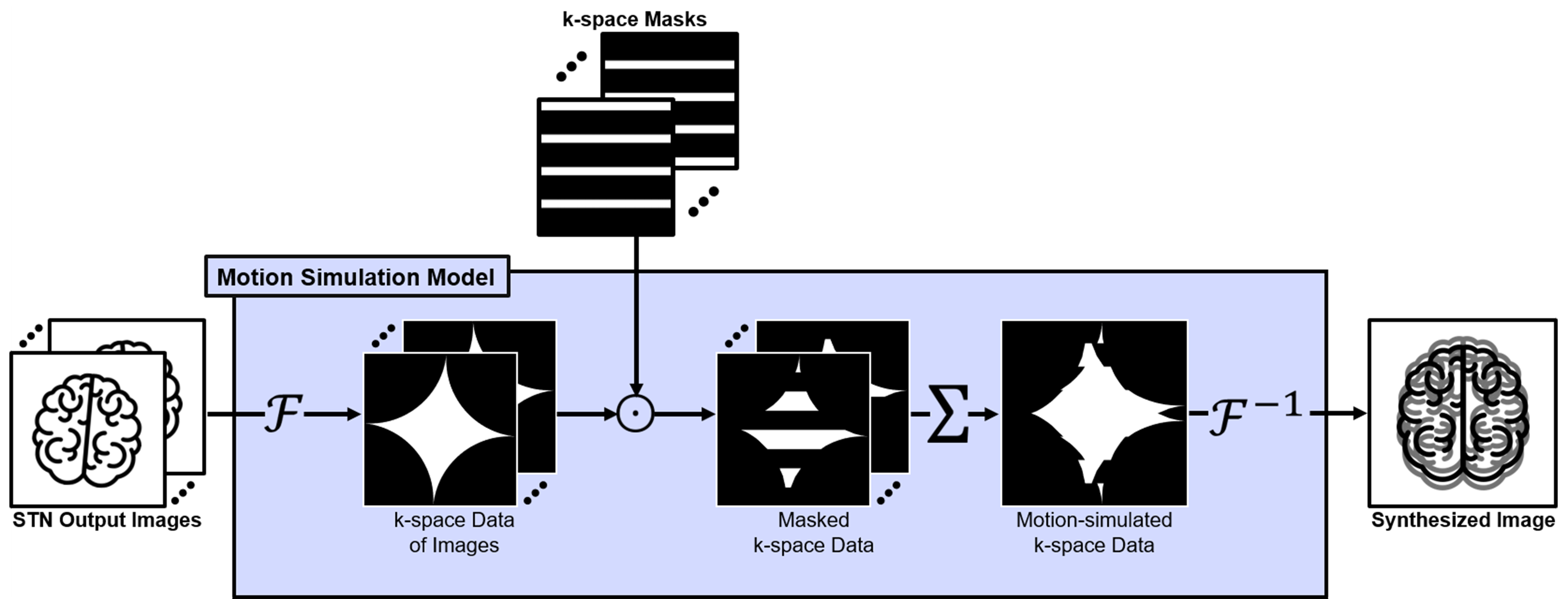
Figure 2. A
motion simulation model with STN output images and k-space masks. The input
images are Fourier transformed and the transformed k-space data are masked by the
input masks. The masked k-space data are summed to be a motion-simulated
k-space data, which is inverse Fourier transformed into the motion-simulated
image.
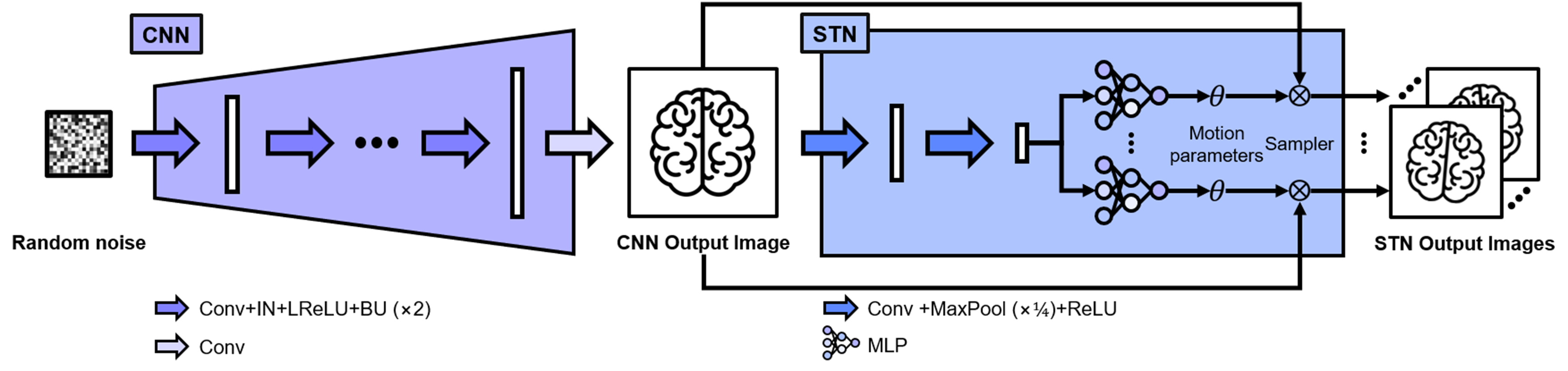
Figure 3. Network
structures of CNN and STN. CNN contains four blocks of convolutional neural
layer (Conv), an instance normalization (BN) layer, a leaky ReLU (LReLU), and a
bilinear up-sampling (BU) layer with a scale of two. Conv is the last layer of
CNN. STN contains two blocks of Conv, a max-pooling (MaxPool) layer with a scale
of four, and ReLU, and $$$N$$$-MLPs that
produce one rotation parameter and two translation parameters that generate $$$N$$$-transformed
images.
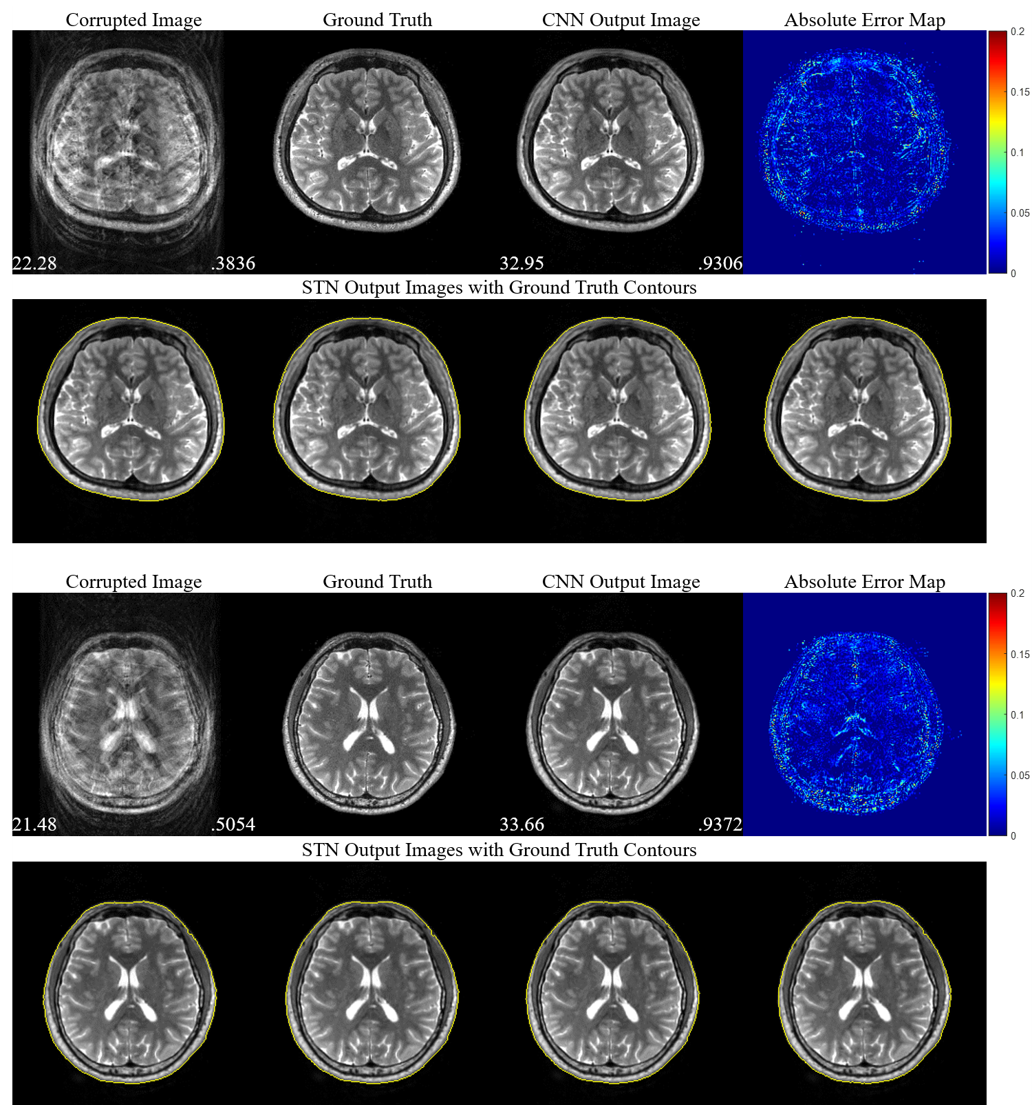
Figure 4.
Visualization of experimental results with cases of three motions (the number
of motion states is four). PSNR (bottom-left) and SSIM (bottom-right) are
provided for motion-corrupted images and motion-corrected (CNN output) images. Absolute
error maps between the corrected images and the ground truth images are magnified
by five. Four transformed images with ground truth contours are shown below.
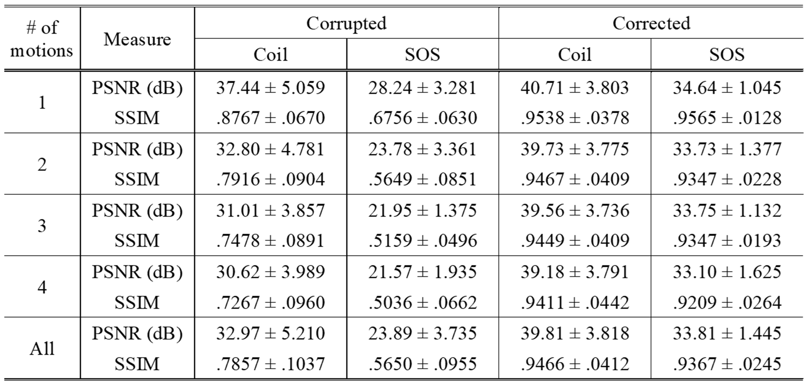
Table 1. Performances on the simulated
dataset with the number of motions from 1 to 4. Averaged PSNR and SSIM compared
to ground truth images are recorded with standard deviations for 32-coil images
(Coil) and sum-of-square images (SOS), separately.
DOI: https://doi.org/10.58530/2023/0352