0351
Stacked UNet-Assisted Joint Estimation for Robust 3D Motion Correction1Dpt. of Medical Biophysics, University of Toronto, Toronto, ON, Canada, 2University Health Network, Toronto, ON, Canada
Synopsis
Keywords: Motion Correction, Motion Correction
We showed that accurate 3D retrospective motion correction of T1w MPRAGE data can be achieved with a UNet-assisted joint estimation algorithm. We compared the proposed method to using the UNet on its own and the standard joint estimation algorithm. Joint estimation (with and without the UNet) outperformed using the stand-alone UNet. The UNet-assisted joint estimation algorithm converged faster than its UNet-free counterpart. We demonstrated the importance of adapting to the changing levels of artifacts over the course of the joint estimation algorithm by sequentially employing different UNets trained for correcting different levels of motion corruption.Introduction
Subject motion remains a major source of image quality degradation in both research and clinical imaging settings. Data-driven retrospective motion correction (RMC) methods [1]–[4] are promising approaches for salvaging corrupted data . A recent RMC method [5] that leveraged both deep learning and classical optimization demonstrated promising 2D motion correction performance. In this work, we demonstrate a robust approach for hybridizing deep learning and classical optimization for 3D motion correction.Methods
Three RMC methods (Fig 1) were implemented and evaluated with simulated motion-corrupted data. Their performance was quantified by the normalized root mean squared error (NRMSE) and structural similarity index (SSIM).Method 1 – 3D Motion Correction with Stacked UNet
To assess the performance of a state-of-the-art deep learning RMC approach, we selected the Stacked UNet with Self-Assisted Priors [6] because of its efficient ability to process 3D MRI data and correct through-plane motion. We trained three separate UNets for correcting mild (UNetmild), moderate (UNetmoderate) and severe (UNetsevere) levels of motion; further information (including the training/testing datasets’ maximum translation/rotation extents) is provided in Data and in Fig 1b.
Method 2 – 3D Joint Image and Motion Estimation
The joint image and motion estimation algorithm [3] (Fig 1a) is derived from the following model of the motion-corrupted MRI signal encoding process [7]:
| | $$s=E_{\theta}m+\eta$$ | $$(1)$$ |
| | $$E_{\theta}=U \mathcal{F}C\theta$$ | $$(2)$$ |
| | $$\hat{m}=argmin_m ||E_{\hat{\theta}}m-s||^2$$ | $$(3)$$ |
| | $$\hat{\theta}=argmin_{\theta} ||E_{\theta}\hat{m}-s||^2$$ | $$(4)$$ |
Method 3 – Stacked UNet-Assisted Joint Image and Motion Estimation
Method 3 extends the framework introduced by Haskell et al [5] for 3D motion correction (Fig 1a). Prior to solving Eq. 3 in each joint estimation step, the corrupted image is passed through the Stacked UNet (Eq. 5) to remove motion artifacts. This pre-processing step decouples Eq. 3 and 4, thereby improving the convergence properties of the joint estimation algorithm [5].
| | $$\hat{m}^*=UNet(\hat{m})$$ | $$(5)$$ |
Data
A dataset of simulated motion-corrupted images was generated from publicly-available, artifact-free 3D T1w MPRAGE data (N = 67 images; 1 mm isotropic; 3T multi-vendor; 12-channel k-space data) [10]. The motion trajectories were randomly generated based on typical head motion characteristics [11], [12]. The retrospective corruption was simulated with an interleaved sampling pattern (SENSE R = 2). Separate training datasets were generated for mild, moderate, and severe levels of motion; please see Fig 1b for further details.
Results
Fig 2 compares the performance of Method 3 with different UNet combinations for a single subject with severe motion corruption (NRMSE: 23.6%; SSIM: 0.80). When using only UNetsevere or UNetmoderate, the image quality improvement plateaus as the algorithm reaches the tail-end of each network’s respective training distribution. When using only UNetmild, the algorithm diverges because the test case is far outside of the network’s training distribution. The sequential combination of all three UNets led to the best motion correction quality; as such, this UNet combination will be used in all subsequent applications of Method 3.Continuing with the same test case, Fig 3 compares the performance of all three methods. Method 1 leads to residual motion artifacts and extensive image blurring. In contrast, Methods 2 and 3 were both able to recover the underlying motion-free image accurately (NRMSE < 3.0%; SSIM $$$\approx$$$ 0.99). Method 2 reached the stopping condition after 1351 iterations, while Method 3 only required 16 iterations (Fig 4a).
Fig 5 shows that Method 3 performed consistently well across the 21 test cases. The minimum and maximum number of iterations required for motion correction were 10 and 20, respectively.
Discussion and Conclusions
We have shown that the joint estimation algorithm can provide accurate and fast 3D motion correction when an appropriate neural network is included. The motion correction quality achieved by joint estimation (Methods 2 & 3) outperforms the performance of using a stand-alone UNet (Method 1). The inclusion of the UNet in the joint estimation algorithm (Method 3) significantly accelerates its convergence rate, corroborating previous findings for 2D motion correction [5].Furthermore, we have demonstrated the benefit of using different UNets in Method 3 to ensure that the training and test dataset distributions remained well-matched over the course of the algorithm. Future work will investigate unrolled training approaches [13]–[15] to tailor the network weights across different joint estimation iterations.
Acknowledgements
No acknowledgement found.References
[1] D. Atkinson, D. L. G. Hill, P. N. R. Stoyle, P. E. Summers, and S. F. Keevil, “Automatic correction of motion artifacts in magnetic resonance images using an entropy focus criterion,” IEEE Trans. Med. Imaging, vol. 16, no. 6, pp. 903–910, 1997, doi: 10.1109/42.650886.
[2] A. Loktyushin, H. Nickisch, R. Pohmann, and B. Schölkopf, “Blind retrospective motion correction of MR images,” Magn. Reson. Med., vol. 70, no. 6, pp. 1608–1618, 2013, doi: 10.1002/mrm.24615.
[3] L. Cordero-Grande, R. P. A. G. Teixeira, E. J. Hughes, J. Hutter, A. N. Price, and J. V. Hajnal, “Sensitivity Encoding for Aligned Multishot Magnetic Resonance Reconstruction,” IEEE Trans. Comput. Imaging, vol. 2, no. 3, pp. 266–280, 2016, doi: 10.1109/tci.2016.2557069.
[4] D. Polak et al., “Scout accelerated motion estimation and reduction (SAMER),” Magn. Reson. Med., vol. 87, no. 1, pp. 163–178, doi: 10.1002/mrm.28971.
[5] M. W. Haskell et al., “Network Accelerated Motion Estimation and Reduction (NAMER): Convolutional neural network guided retrospective motion correction using a separable motion model,” Magn. Reson. Med., vol. 82, no. 4, pp. 1452–1461, 2019, doi: 10.1002/mrm.27771.
[6] M. A. Al-masni et al., “Stacked U-Nets with self-assisted priors towards robust correction of rigid motion artifact in brain MRI,” NeuroImage, vol. 259, p. 119411, Oct. 2022, doi: 10.1016/j.neuroimage.2022.119411.
[7] P. G. Batchelor, D. Atkinson, P. Irarrazaval, D. L. G. Hill, J. Hajnal, and D. Larkman, “Matrix description of general motion correction applied to multishot images,” Magn. Reson. Med., vol. 54, no. 5, pp. 1273–1280, 2005, doi: 10.1002/mrm.20656.
[8] K. P. Pruessmann, M. Weiger, M. B. Scheidegger, and P. Boesiger, “SENSE: Sensitivity encoding for fast MRI,” Magn. Reson. Med., vol. 42, no. 5, pp. 952–962, Nov. 1999, doi: 10.1002/(SICI)1522-2594(199911)42:5<952::AID-MRM16>3.0.CO;2-S.
[9] J. Nocedal and S. J. Wright, Numerical optimization, 2nd ed. New York: Springer, 2006.
[10] R. Souza et al., “An open, multi-vendor, multi-field-strength brain MR dataset and analysis of publicly available skull stripping methods agreement,” NeuroImage, vol. 170, pp. 482–494, Apr. 2018, doi: 10.1016/j.neuroimage.2017.08.021.
[11] H. Eichhorn et al., “Characterisation of Children’s Head Motion for Magnetic Resonance Imaging With and Without General Anaesthesia,” Front. Radiol., vol. 1, 2021, doi: 10.3389/fradi.2021.789632.
[12] A. T. Hess, F. Alfaro-Almagro, J. L. R. Andersson, and S. M. Smith, “Head movement in UK Biobank, analysis of 42,874 fMRI motion logs,” presented at the ISMRM 2022 Workshop on Motion Detection & Correction, Oxford, England, 2022.
[13] K. Hammernik et al., “Learning a variational network for reconstruction of accelerated MRI data,” Magn. Reson. Med., vol. 79, no. 6, pp. 3055–3071, Nov. 2017, doi: 10.1002/mrm.26977.
[14] J. Schlemper, J. Caballero, J. V. Hajnal, A. N. Price, and D. Rueckert, “A Deep Cascade of Convolutional Neural Networks for Dynamic MR Image Reconstruction,” IEEE Trans. Med. Imaging, vol. 37, no. 2, pp. 491–503, 2018, doi: 10.1109/TMI.2017.2760978.
[15] V. Monga, Y. Li, and Y. C. Eldar, “Algorithm Unrolling: Interpretable, Efficient Deep Learning for Signal and Image Processing,” IEEE Signal Process. Mag., vol. 38, no. 2, pp. 18–44, Mar. 2021, doi: 10.1109/MSP.2020.3016905.
Figures
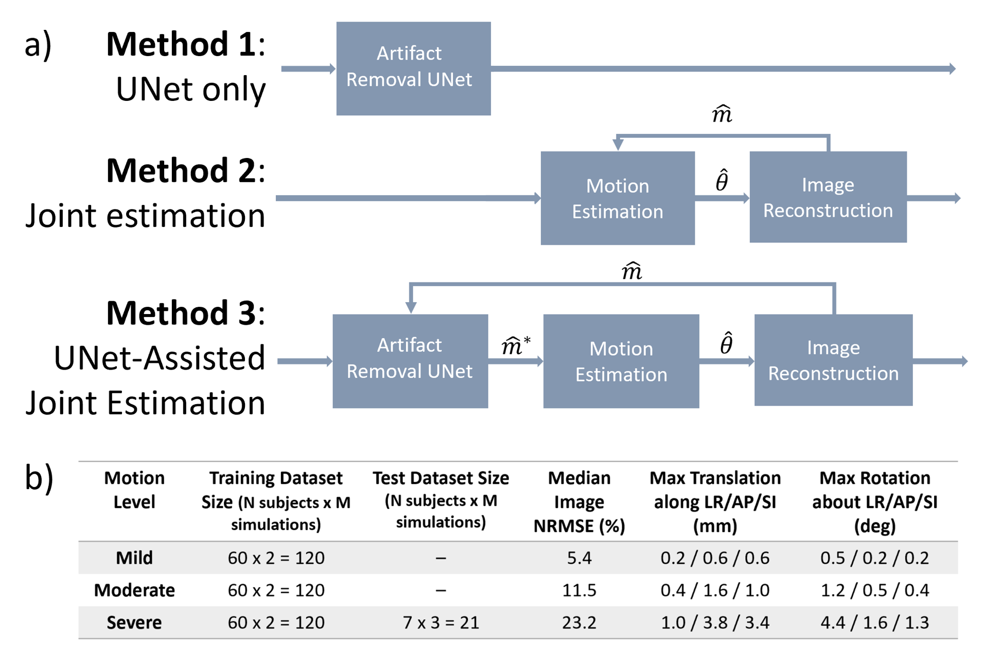
Figure 1. a) Method 1 consists of the Stacked UNet with Self-Assisted Prior, which was trained with SSIM loss and the Adam optimizer. Method 2 is the 3D joint estimation algorithm. Method 3 combines the UNet with the joint estimation algorithm. b) Three different UNet training datasets were generated for different levels of motion corruption.
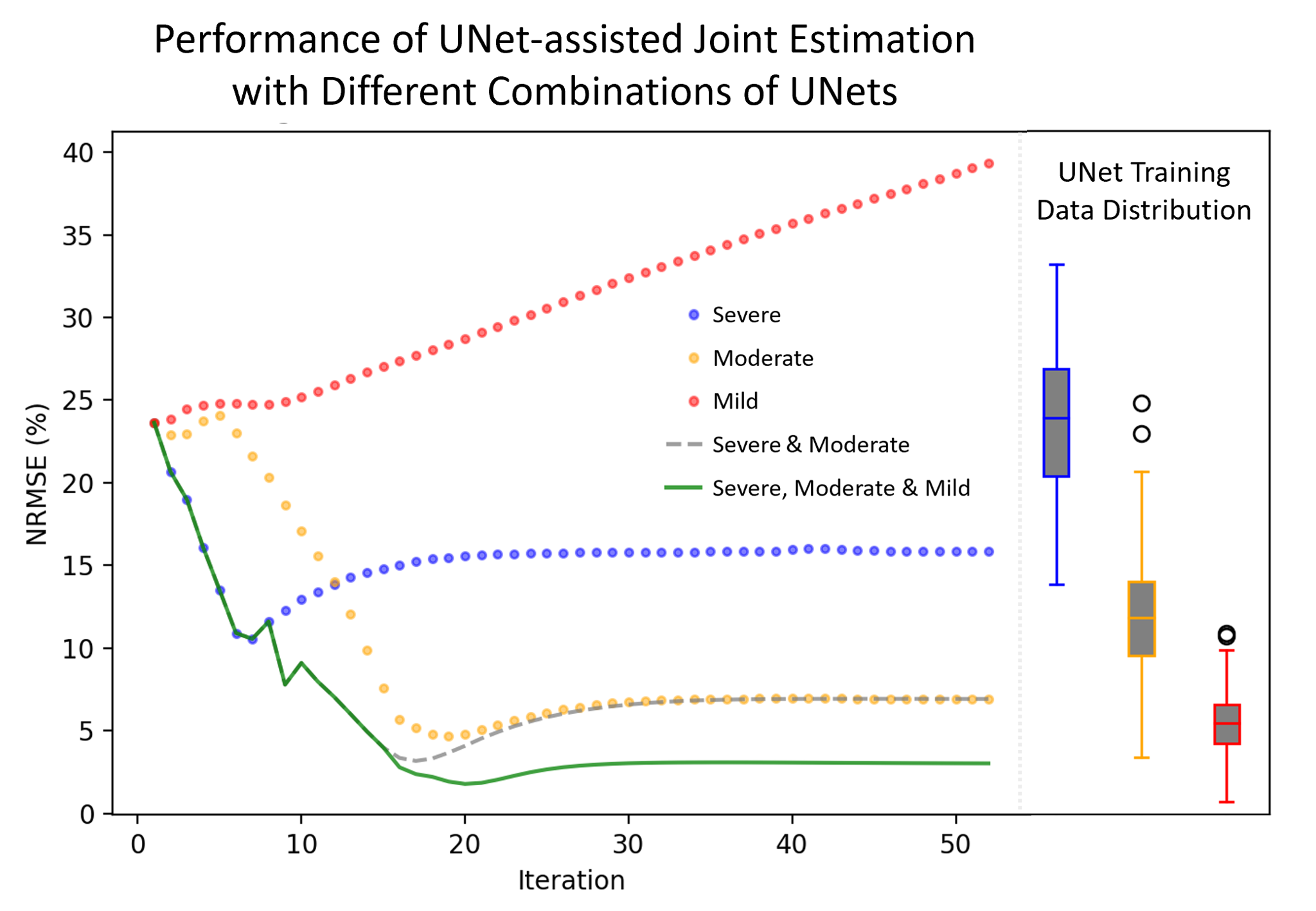
Figure 2. Left subplot: A comparison of the performance of Method 3 with the following UNet combinations: using only UNetsevere; using only UNetmoderate; using only UNetmild; using UNetsevere for iteration 1 – 6 and UNetmoderate for iterations >= 7; and using UNetsevere for iteration 1 – 6, UNetmoderate for iterations 7 – 13, and UNetmild for iterations >= 14. Right subplot: A comparison of the NMRSE distribution for the severe, moderate, and mild training datasets.
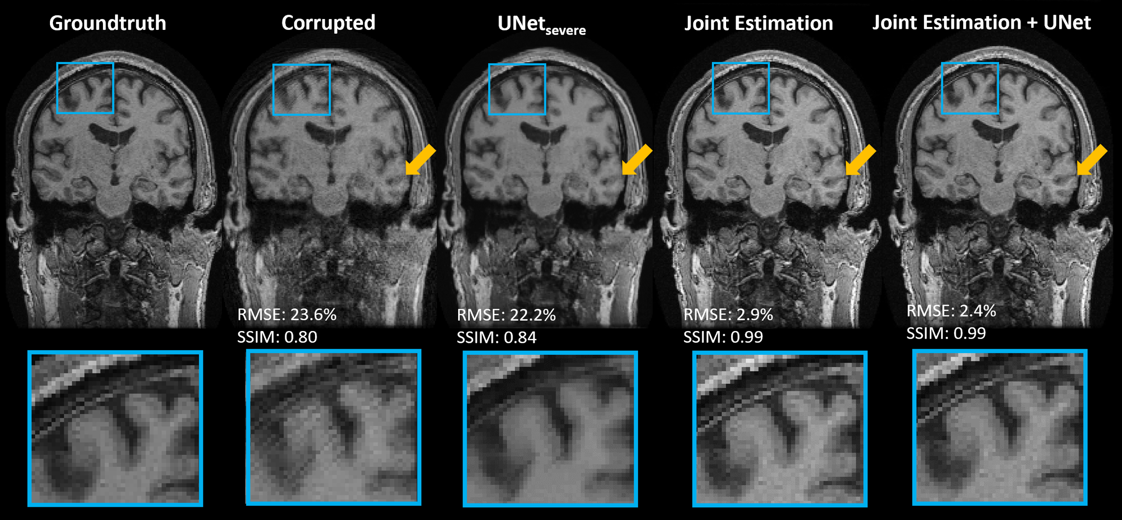
Figure 3. A comparison of Methods 1, 2 and 3 for a test case with a severe level of simulated motion corruption. The coronal view is shown to demonstrate the through-plane correction achieved by the three methods. The blue box highlights a region with strong ghosting in the corrupted image, while the yellow arrow highlights a region where the UNet exhibited strong image blurring.
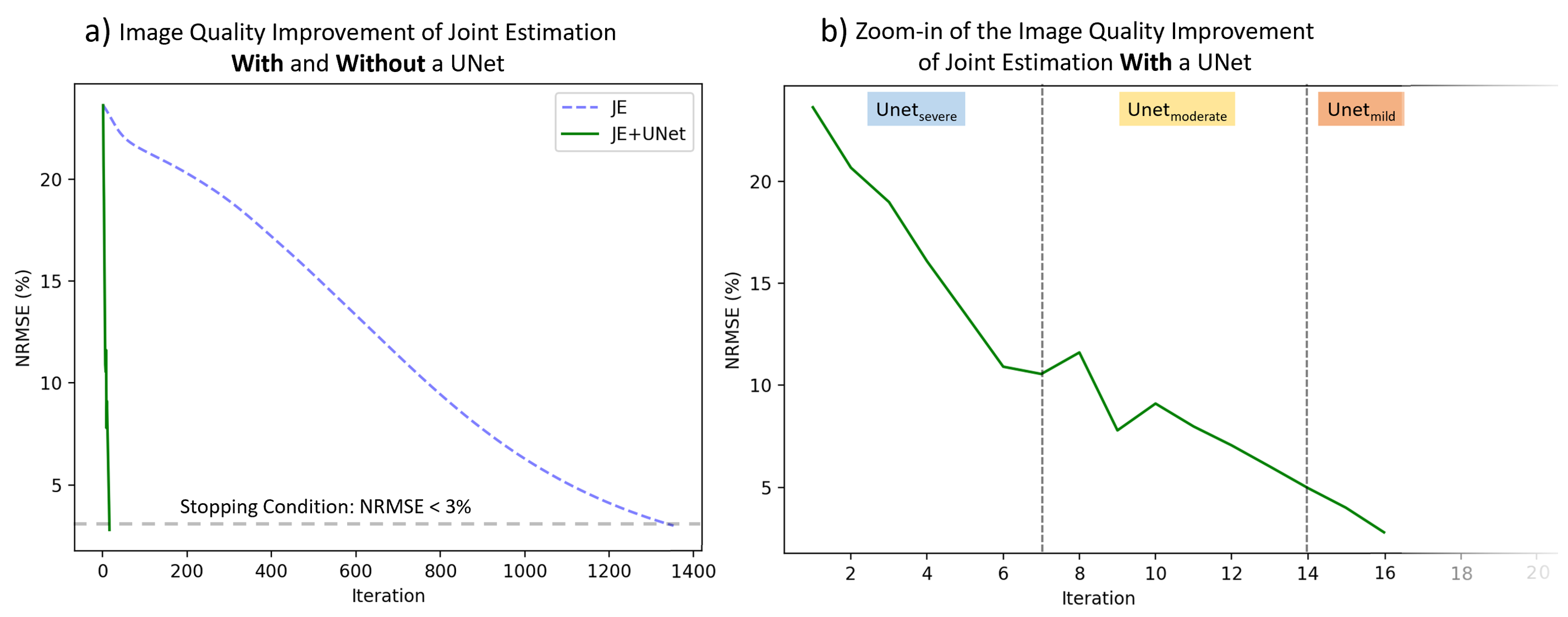
Figure 4. a) A comparison of the trajectory of image quality improvement of Method 2 (Joint Estimation) and Method 3 (UNet-Assisted Joint Estimation). b) A zoom-in of the image quality trajectory for Method 3, with an illustration of the range of iterations at which different UNets were used. Please note that the x-axis scale (i.e., number of iterations) is much smaller in b).
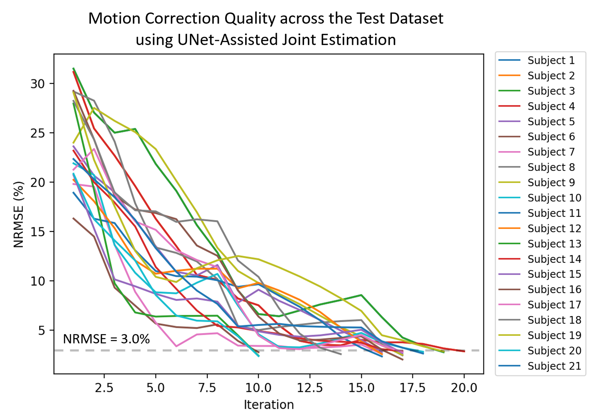
Figure 5. Assessing the performance of Method 3 across N = 21 test cases, with simulated severe motion corruption (NRMSEmedian: 23.6%, NRMSEmin: 16.3%, NRMSEmax: 31.5%). The dashed grey line demarcates the algorithm’s stopping condition (NRMSE < 3.0%).