0350
Retrospective motion correction and reconstruction for clinical 3D brain MRI protocols with a reference contrast
Gabrio Rizzuti1, Tim Schakel1, Niek Huttinga1, Tristan van Leeuwen2, and Alessandro Sbrizzi1
1Universitair Medisch Centrum Utrecht, Utrecht, Netherlands, 2Centrum Wiskunde & Informatica, Amsterdam, Netherlands
1Universitair Medisch Centrum Utrecht, Utrecht, Netherlands, 2Centrum Wiskunde & Informatica, Amsterdam, Netherlands
Synopsis
Keywords: Motion Correction, Brain, brain, clinical protocols, motion correction, retrospective correction
We discuss the application of a novel 3D retrospective rigid motion correction and reconstruction scheme to in-vivo data for clinical 3D brain protocols. The correction scheme leverages multiple scans contained in a typical MR session, of which some are corrupted by motion but at least one scan may be devoid of motion artifacts. The uncorrupted scan is then used as a reference to regularize a generalized rigid-motion registration problem. We discuss the potential of the proposed algorithm with a prospective in-vivo study.Introduction
In a typical MR session, several contrasts are acquired. Due to the sequential nature of the data acquisition process, the patient may experience some discomfort at some point during the session, and start moving. Hence, it is quite common to have MR sessions where some contrasts are well-resolved, while other contrasts exhibit motion artifacts. Instead of repeating the scans that are corrupted by motion, we introduce a reference-guided retrospective motion correction scheme that takes advantage of the motion-free scans, based on a generalized rigid registration routine. This work builds upon a previous study6, and extends the method introduced therein to 3D and to prospective in-vivo data. We focus on existing clinical 3D brain protocols based on Cartesian sampling, with no need for dedicated motion-resilient acquisitions4. Ideally, we depict the following scenario: a trained technician should indicate the corrupted and the motion-free scans. Afterwards, the post-processing of the corrupted scan discussed in this work will eliminate the motion artifacts. We demonstrate the feasibility of the proposed method on 3D clinical protocols for brain MRI with volunteer data and different types of motion.Mathematical formulation
The proposed method aims at estimating the time-dependent rigid motion parameter evolution $$$\pmb{\theta}^t$$$, while removing its effects from the otherwise motion-corrupted 3D image $$$\mathbf{u}$$$. The temporal coordinate $$$t$$$ can be equated to the phase-encoding coordinate in the $$$k$$$-space, ordered by the acquisition sequence. Note that no intra-readout motion is assumed. The method is summarized by the following minimization problem:$$\min_{\mathbf{u}\in C(\mathbf{v}),\pmb{\theta}^1,\ldots,\pmb{\theta}^{n_t}}\mathcal{J}(\mathbf{u},\pmb{\theta}^1,\ldots,\pmb{\theta}^{n_t})=\sum_t \dfrac{1}{2}||\mathcal{F}(\pmb{\theta}^t)\mathbf{u}-\mathbf{d}^t||^2+\lambda\mathcal{R}_{\theta}(\pmb{\theta}^1,\ldots,\pmb{\theta}^{n_t}).$$
The motion-perturbed Fourier transform $$$\mathcal{F}(\pmb{\theta})$$$ computes the Fourier coefficients associated to each $$$k$$$-space sample of the rotated readout line according to $$$\pmb{\theta}$$$ (hence, we require the non-uniform Fourier transform) and it includes the phase-shift caused by the corresponding translation. The (coil-resolved) data is represented by $$$\mathbf{d}$$$, and can be obtained by a preliminary SENSE reconstruction of the corrupted data, followed by the conventional Fourier transform. Note that this step can be just performed by the scanner reconstruction in the case when no compressed-sensing reconstruction is employed. The motion parameter regularization term $$$\mathcal{R}_{\theta}$$$ enforces time-wise smoothness.
The central aspect of the method is the regularization procedure encapsulated by the constraint set $$$C(\mathbf{v})=\{\mathcal{R}_u(\mathbf{u};\mathbf{v})\le\varepsilon\}$$$ (for a prescribed regularization level $$$\varepsilon$$$), where $$$\mathbf{v}$$$ is a given contrast with no motion artifacts. The reconstruction regularization term $$$\mathcal{R}_u(\mathbf{u};\mathbf{v})$$$ is defined by the weighted total-variation (TV) norm5,6
$$\mathcal{R}_u(\mathbf{u};\mathbf{v})=||(\mathrm{I}-\Pi(\mathbf{v}))\nabla\mathbf{u}||_{2,1},\quad\Pi(\mathbf{v})=\widehat{\nabla\mathbf{v}}\,\widehat{\nabla\mathbf{v}}^{\mathrm{H}},$$
where $$$\widehat{\nabla\mathbf{v}}$$$ is the normalized gradient field of $$$\mathbf{v}$$$. This term will promote a contrast whose gradient field will align with the one of $$$\mathbf{v}$$$, thus enforcing structural similarity.
The current CPU implementation of the method for a 256x256x256 3D image requires less than 2 hours. Future work will quantify the gains in computational time of a GPU implementation.
Experiment description
In order to test our proposed method, a healthy volunteer was scanned on a 1.5 T Philips Ingenia scanner using a 15-channel head coil. We prompt the volunteer to move multiple times throughout the acquisition phase of the scan, while laying still in between our instructions. The induced target motion is therefore step-wise constant. The severity of the motion corruption increases with the number of rigid motions performed, so that we can test the robustness of the motion correction with respect to the "complexity" of the motion.We induce three motion corruption levels corresponding to (i) a single change of position (Figure 1), (ii) two changes of position (Figure 2), and (iii) 5 changes of positions (Figure 3). We consider the following specifications:
- corrupted volume: T2-FLAIR weighted contrast, 3D Turbo Spin Echo, acquisition resolution 1.2 mm, field of view 230x230x238 mm3, TR/TE 4800/320 ms, flip angle 90o, scan duration 346 s;
- reference volume: T1 weighted contrast, 3D Fast Field Echo, acquisition resolution 1 mm, field of view 230x230x238 mm3, TR/TE 78/36 ms, TSE factor 224, flip angle 8o, scan duration 182 s.
Discussion
The experiments for 3D in-vivo data based on standard clinical protocols show that blind motion correction is highly inadequate, so that leveraging prior information is paramount to the success of the correction. The robustness of the method was investigated with respect to the motion complexity. As evidenced by Figures 1-3, the proposed method consistently ameliorates the corrupted scan. Furthermore, the quality indexes based on PSNR and SSIM shows only a modest decrease in correction quality as a function of motion complexity (Figure 4). While this is somewhat expected, future applications to patient data will ultimately clarify whether the proposed correction scheme satisfies the radiological requirements.Conclusions
We presented a prospective in-vivo study to test the potential of a recently proposed motion correction scheme6 that leverages a motion-free contrast as an anatomical reference. The experiments highlight the effectiveness of using a motion-free guide in removing motion artifacts. We demonstrate the applicability of the method to clinically applied 3D acquisitions, with no need to resort to specialized motion-resilient acquisitions.Acknowledgements
This publication is part of the project "Reducing re-scans in clinical MRI exams'' (with project number 104022007 of the research program "IMDI,Technologie voor bemensbare zorg: Doorbraakprojecten'') which is financed by The Netherlands Organization for Health Research and Development(ZonMW). The project is also supported by Philips Medical Systems Netherlands BV.References
- Zaitsev, M., Maclaren, J., and Herbst, M. (2015). Motion artifacts in MRI: A complex problem with many partial solutions. Journal of MagneticResonance Imaging, 42(4), 887-901.
- Godenschweger, F., Kägebein, U., Stucht, D., Yarach, U., Sciarra, A., Yakupov, R., and Speck, O. (2016). Motion correction in MRI of the brain.Physics in Medicine & Biology, 61(5), R32.
- Loktyushin, A., Nickisch, H., Pohmann, R., and Schölkopf, B. (2013). Blind retrospective motion correction of MR images. Magnetic resonance inmedicine, 70(6), 1608-1618.
- Cordero‐Grande, L., Ferrazzi, G., Teixeira, R. P. A., O'Muircheartaigh, J., Price, A. N., and Hajnal, J. V. (2020). Motion ‐ corrected MRI with DISORDER:Distributed and incoherent sample orders for reconstruction deblurring using encoding redundancy. Magnetic resonance in medicine, 84(2),713-726.
- Ehrhardt, M. J., and Betcke, M. M. (2016). Multicontrast MRI reconstruction with structure-guided total variation. SIAM Journal on Imaging Sciences, 9(3), 1084-1106.
- Rizzuti, G., Sbrizzi, A., and van Leeuwen, T. (2022). Joint Retrospective Motion Correction and Reconstruction for Brain MRI With a Reference Contrast. IEEE Transactions on Computational Imaging, 8, 490-504.
Figures
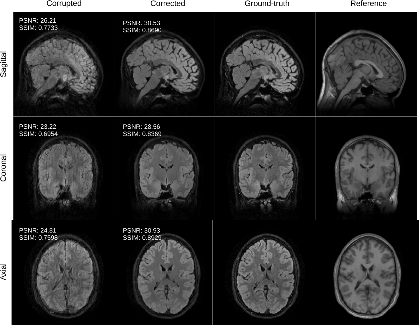
Figure 1: the volunteer is instructed to suddenly change its position once during the scan. We compare the conventional reconstruction (corrupted) with the output of the proposed retrospective motion correction scheme (corrected). The corrected slices compare favorably with the ground-truth both in terms of quality metrics PSNR and SSIM. We also show the motion-free reference employed by our algorithm.
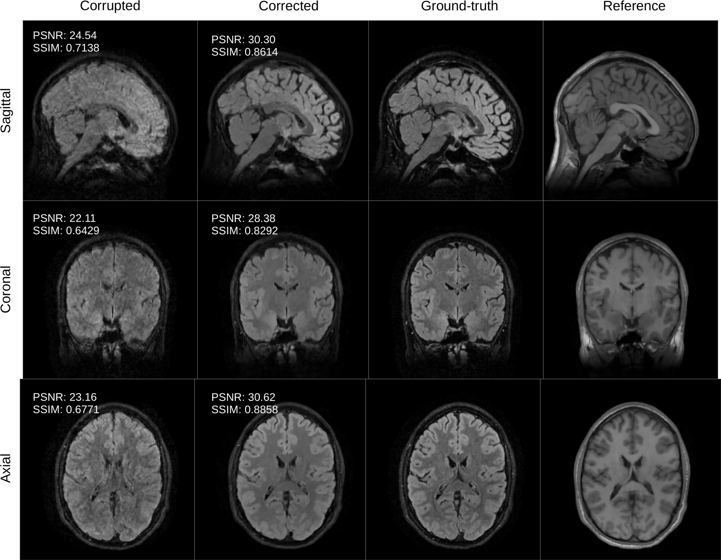
Figure 2: the volunteer is instructed to suddenly change its position twice during the scan. We compare the conventional reconstruction (corrupted) with the output of the proposed retrospective motion correction scheme (corrected). The corrected slices compare favorably with the ground-truth both in terms of quality metrics PSNR and SSIM. We also show the motion-free reference employed by our algorithm.
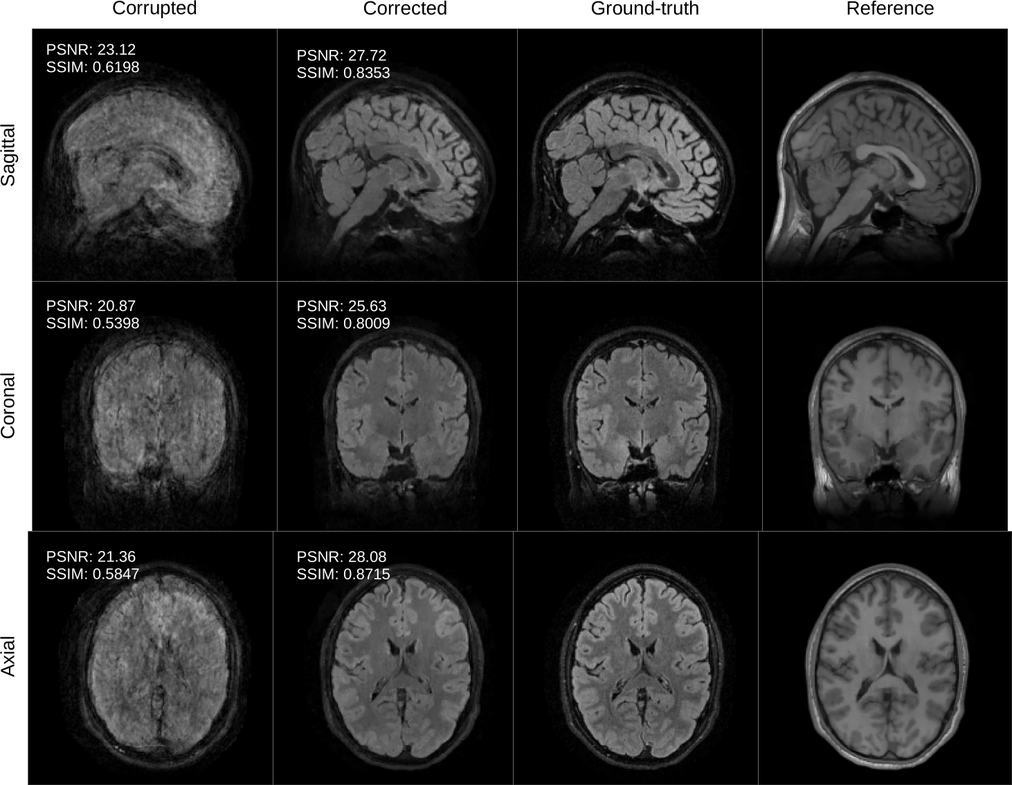
Figure 3: the volunteer is instructed to suddenly change its position 5 times during the scan. We compare the conventional reconstruction (corrupted) with the output of the proposed retrospective motion correction scheme (corrected). The corrected slices compare favorably with the ground-truth both in terms of quality metrics PSNR and SSIM. We also show the motion-free reference employed by our algorithm.
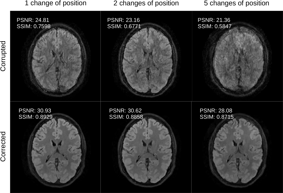
Figure 4: Summary of the motion correction results presented in Figures 1-3. Here, we highlight the decreasing quality of the motion correction as a function of motion complexity for a fixed axial slice. Nevertheless, the corrected results are relatively stable with respect to motion severity.
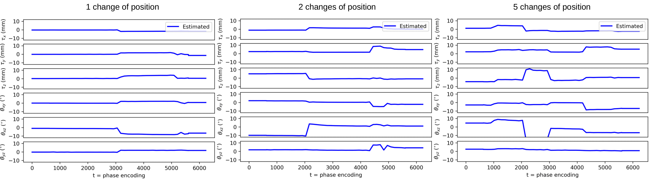
Figure 5: Estimated 3D motion parameters as a function of time $$$t$$$ for the experiments presented in Figures 1-3, comprising translations $$$\tau_x,\tau_y,\tau_z$$$ and rotation angles $$$\theta_{xy},\theta_{xz},\theta_{yz}$$$ (xy = axial plane, xz = coronal plane, yz = sagittal plane).
DOI: https://doi.org/10.58530/2023/0350