0319
Direct measurement of luminal diffusivity in prostate: Prostate diffusion at an echo time of 400 ms.1New York University Grossman School of Medicine, New York, NY, United States, 2Microstructure Imaging, INC, New York, NY, United States
Synopsis
Keywords: Prostate, Prostate, Diffusion
We showcase, for the first time, a direct/model-free measurement of luminal diffusivity in prostate, where ADC contrast no longer contains the cellular contribution, and only describes features of the glandular lumen, which prominently shrink with increasing Gleason score. We show that with a 4m30s protocol, the luminal volume fraction, cellular and luminal diffusivities can be obtained with high accuracy/precision at 1.5x1.5x3.0 mm3, suggesting that this approach can feasibly replace the current state-of-the-art, ~6 minute, prostate diffusion acquisition.Introduction
Echo-time($$$T_E$$$)$$$\,$$$dependence is a major covariate influencing the image quality and contrast of prostate diffusion images, where an increase in$$$\,T_E\,$$$leads to an increase in the apparent diffusion coefficient,$$$\,ADC$$$1-3. This $$$ADC$$$ increase is due to selective suppression of low$$$\,T_2\,$$$cellular tissue signal and preservation of the high$$$\,T_2\,$$$luminal signal. An MRI measurement specific to the luminal compartment may be incredibly valuable due to the prominent luminal changes with Gleason grade,4 which include changes in diameter, anisotropy, and volume fraction. Since this observation, modeling approaches such as rVERDICT,5 Hybrid Multi-Dimensional Imaging,6 Diffusion-Relaxation Spectrum imaging,7 and Ref.1 incorporated maximum$$$\,T_E\,$$$measurements,$$$\,T_E^{Max}$$$, of $$$[80,100,120,\,\mathrm{and }180]\,\mathrm{ms}$$$, respectively. In each of these works, the choice of$$$\,T_E^{Max}\,$$$is relatively short, considering that the long$$$\,T_2\,$$$of the peripheral-zone of the prostate is reported8,9 to be greater than $$$300$$$ ms. The reason why these approaches carefully avoided long$$$\,T_E\,$$$s, was that the exponential decay of$$$\,T_2\,$$$weighting is further compounded by the exponential decay of diffusion weighting, which heavily suppresses the little signal available in the prostate. Due to these overbearing SNR limitations, diffusion in the luminal compartment has never been observed directly and has only been inferred through modeling. In this abstract, we leverage the random matrix theory (RMT) reconstruction10-13 to dramatically increase the SNR of a conventional prostate protocol. Following RMT reconstruction, we can observe$$$\,ADC\,$$$at$$$\,T_E=400\,\mathrm{ms}$$$, where the cellular diffusivity has been entirely suppressed and the diffusion contrast originates only from the lumen.Methods
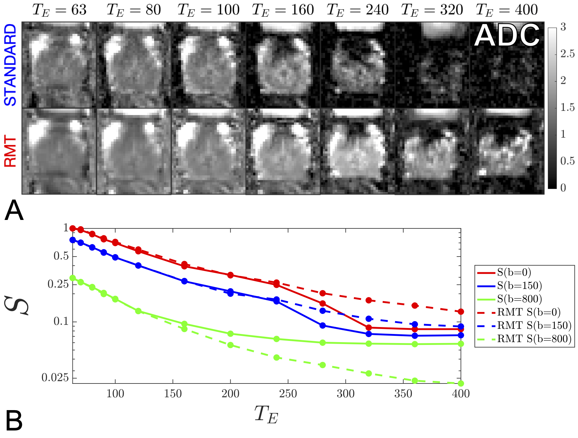
Acquisition & ReconstructionA 31 y/o volunteer was imaged using a multi-parametric diffusion pulsed gradient spin echo acquisition, with$$$\,[4\,b=0,\,3\,b=150\,s/mm^2,\,$$$and$$$\,8\,b=800\,s/mm^2]\,$$$over non-collinear directions with$$$\,TR=[10,\,10,\,10,\,10,\,10,\,10,\,10,\,11,\,12.5,\,14.0,\,15.4,\,16.8,\,18.2]\,s\,$$$and$$$\,T_E=[ 63,\,70,\,80,\,90,\,100,\,120,\,160,\,200,\,240,\,280,\,320,\,360,\,400]\,\mathrm{ms}$$$. The acquisition was performed on a Siemens 3T Magnetom PRISMA system with 20-receive channels enabled between the 8-channel phased array surface coil and the 24-channel spine matrix coil. Other imaging parameters include $$$FOV=200\times\,200\times\,90\,mm^3$$$, $$$1.5\times\,1.5\times\,3.0\,mm^3$$$ voxel size, iPAT=2 reconstructed with GRAPPA, partial-Fourier=6/8 filled with POCS, phase-oversampling=50%, bandwidth=1325$$$\,$$$Hz/pixel, the 20 coil images were combined via adaptive combination.14 The random matrix theory reconstruction10-13 was performed by combining$$$\,20\,$$$coil elements with$$$\,195\,$$$measurements ($$$15\,$$$ diffusion directions $$$\times$$$ $$$13\,T_E$$$s). RMT was used to increase the SNR of diffusion images such that$$$\,ADC\,$$$could be observed with minimal Rician bias [Fig.1].
Modeling
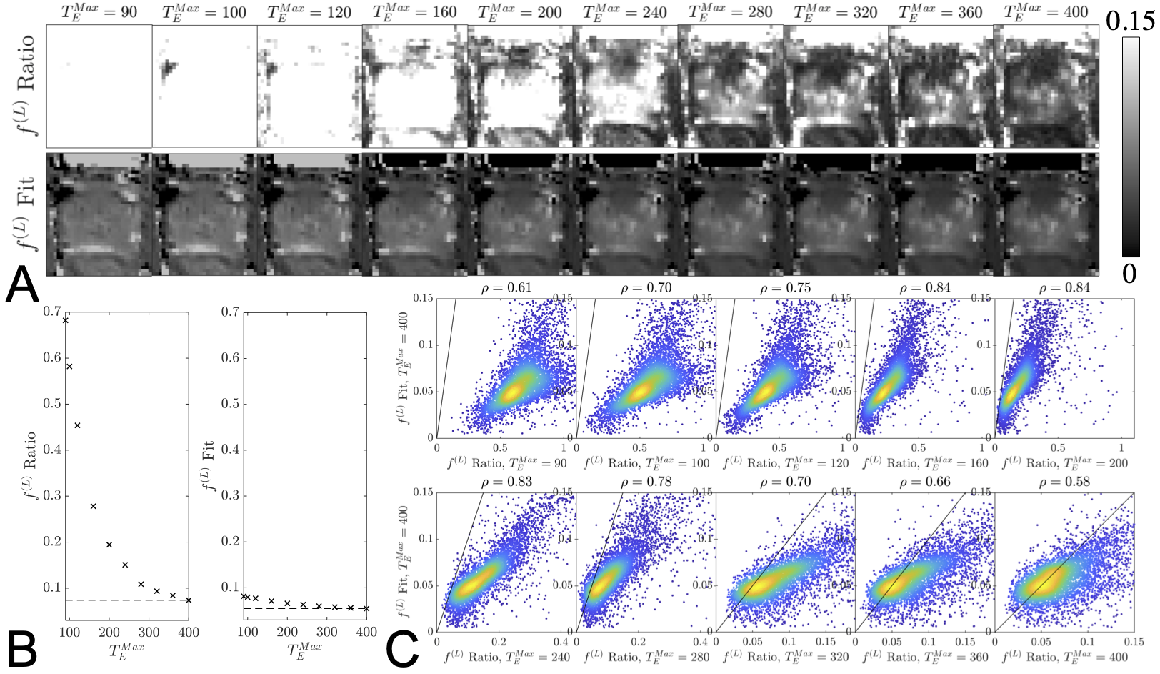
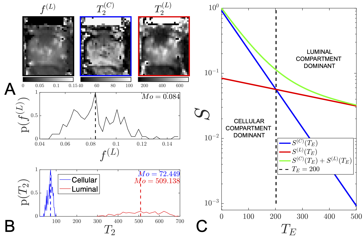
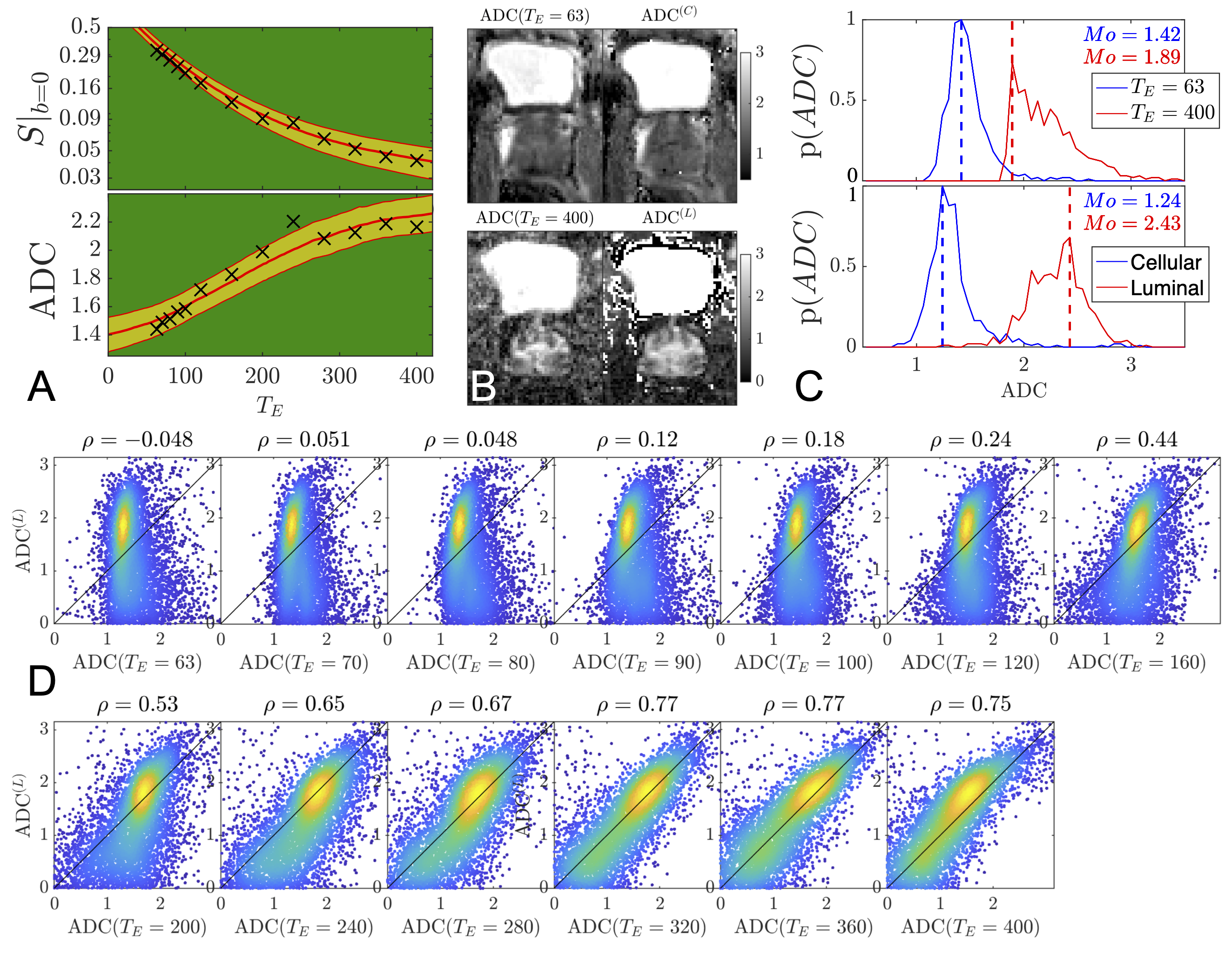
We estimated the unweighted signal,$$$\,S|_{b=0}(T_E)$$$,$$$\,$$$and$$$\,ADC(T_E)$$$, at each$$$\,T_E$$$, using weighted linear least squares excluding the measured$$$\,b=0\,$$$measurements to avoid bias from IVIM.$$$\,S|_{b=0}(T_E)\,$$$was then used to determine$$$\,4\,$$$parameters of a biexponential relaxation model: proton density, $$$\,S|_{b,T_E=0}$$$, the luminal volume fraction,$$$\,f^{(L)}$$$, and cellular (fast) and luminal (slow)$$$\,T_2\,$$$components,$$$\,T_2^{(C)}\,$$$and$$$\,T_2^{(L)}$$$, respectively:$$S|_{b=0}(T_E)=S|_{b,T_E=0}\bigg(\underbrace{(1-f^{(L)})e^{-T_E/T_2^{(C)}}}_C+\underbrace{f^{(L)}e^{-T_E/T_2^{(L)}}}_L\bigg)\,\,\,\,\,\,\,\,\,\,(1)$$A machine learning (ML) polynomial regression approach14,15 (order=3) was used to learn the mapping from a biexponential signal with Rician noise to model parameters, using uniform priors:$$$\,f^{(L)}=[0,0.15]$$$,$$$\,T_2^{(C)}=[0,100]$$$,$$$\,T_2^{(L)}=[0,1000]$$$.To confirm the estimate of$$$\,f^{(L)}\,$$$from biexponential modeling, we employ a ratio approach:$$f^{(L)}=\frac{S|_{b=0}(T_E^{Max})}{S|_{b,T_E=0}}\approx\frac{S|_{b=0}(T_E^{Max})}{S|_{b=0}(T_E=63)}\,\,\,\,\,\,\,\,\,\,(2)$$which states that at sufficiently long$$$\,T_E$$$, the cellular compartment will be suppressed and the remaining signal contribution will be mostly from the luminal compartment, when normalized by signal at the shortest available$$$\,T_E$$$.Using the fit results of Equation(1), we generate$$$\,T_E\,$$$-specific weights,$$$\,W(T_E),\,$$$to calculate cellular and luminal$$$\,ADC$$$s,$$$\,\,ADC^{(C)}\,$$$and$$$\,ADC^{(L)}$$$, using linear inversion:$$ADC(T_E)=W(T_E)\cdot\mathrm{}ADC^{(C)}+(1-W(T_E)\cdot\mathrm{}ADC^{L},\,\,\,\,\,\,\,\,\,\mathrm{where}\,\,\,\,W(T_E)=\frac{C}{C+L}\,\,\,\,\,\,\,\,\,\,(3)\\\mathrm{pinv}\left(\begin{matrix}W(T_{E_1})&1-W(T_{E_1})\\W(T_{E_2})&1-W(T_{E_2})\\\vdots&\vdots\\W(T_{E_N})&1-W(T_{E_N})\end{matrix}\right)\begin{bmatrix}\mathrm{ADC}(T_{E_1})\\\mathrm{ADC}(T_{E_2})\\\vdots\\\mathrm{ADC}(T_{E_N})\end{bmatrix}=(\mathrm{ADC}^{(C)}\,\,\,\,\mathrm{ADC}^{(L)})\,\,\,\,\,\,\,\,\,\,(4)$$
Results
The RMT reconstruction increases the SNR by$$$\,\,5.6x\,$$$over the standard reconstruction within the region of the prostate, thereby enabling the observation of $$$ADC$$$ at long echo times [Fig.1].From the unweighted signal$$$\,\,S|_{b=0}(T_E)$$$, we observe that estimates of$$$\,\,f^{(L)}\,$$$from biexponential fitting and the ratio method [2] coincide for$$$\,\,T_E>320\,$$$ms [Fig.2]. This serves as a consistency check on our rationale for Equation(2). The values of $$$f^{(L)}$$$ indicate that several modeling approaches5-7 have overestimated$$$\,\,f^{(L)}\,(0.2-0.4)\,$$$due to their limited range of$$$\,\,T_E\,$$$and conflation with diffusion-weighting. The results from this abstract are in agreement with modeling approaches focusing exclusively on relaxometry$$$\,\,f^{(L)}\,(0.05-0.15)$$$.8,9
From this extended range, we find that at$$$\,T_E=400\,$$$ms, the luminal compartment has$$$\,10.4x\,$$$the amount of signal than the cellular compartment [Fig.3], whereas at$$$\,T_E=63\,$$$ms the cellular compartment signal was$$$\,5.2x\,$$$larger than the luminal compartment, [Fig.3]. Considering diffusion, we find that the$$$\,ADC(T_E)\,$$$increases linearly with $$$T_E$$$ until $$$200$$$ ms, after which$$$\,ADC(T_E)\,$$$asymptotically converges towards$$$\,ADC^{(L)}\,$$$, [Fig.4].
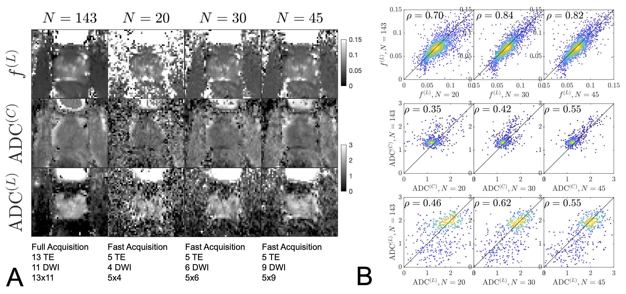
By subsampling images from the full protocol and redoing the RMT reconstruction for the abbreviated sampling scheme [Fig.5], we find that accurate$$$\,f^{(L)}$$$,$$$\,ADC^{(C)}$$$, and$$$\,ADC^{(L)}\,$$$parametric maps can be obtained with only $$$20$$$ images. Sampling schemes with more images improve SNR and precision, but do not offer substantial improvements to accuracy.
Discussion
We speculate that the luminal $$$ADC$$$ will outperform the cellular $$$ADC$$$ in prostate cancer assessment. This speculation has been supported through the observation17 of$$$\,f^{(L)}\,$$$from luminal water imaging outperforming $$$ADC(T_E=72\mathrm{ms})$$$ for differentiating low/high grade prostate cancers. Diffusion weighting should further amplify the features of luminal compartment as it would not only be sensitive to$$$\,f^{(L)}\,$$$, but also be reveal sensitive towards the luminal microstructure,1 representing luminal geometry, diameters, and perhaps exchange.By leveraging RMT,10-13 the in-line averages performed for typical clinical protocols may be replaced with variable$$$\,\,T_E\,$$$acquisitions to generate the above parameter maps. Assuming$$$\,T_R=6\,s\,$$$, the abbreviated protocol$$$\,(N = 45)$$$, [Fig.5], can be acquired in $$$4\mathrm{m}30\mathrm{s}$$$, which is faster than the $$$5\mathrm{m}41\mathrm{s}$$$, $$$1.7\times\,1.7\times\,3.0$$$ voxel size, single$$$\,T_E\,$$$diffusion acquisition suggested as the state-of-the-art acquisition from PIRADsv2.1.18
Conclusion
Using RMT, we have been able explore a previously unattainable region of parameter space at high$$$\,T_E\,$$$to directly measure the$$$\,ADC\,$$$contribution from the luminal compartment. We found strong agreement with measured and estimated$$$\,ADC^{(L)}$$$, offering validation for the biophysical picture of two prostate compartments with radically different$$$\,T_2\,$$$values.Acknowledgements
This work was supported by the NIH under awards: R01NS088040 (NINDS), R41CA257624 (NCI), R01EB027075 (NIBIB), and by the Center of Advanced Imaging Innovation and Research (CAI2R, www.cai2r.net), a NIBIB Biomedical Technology Resource Center: P41EB017183.References
1. Lemberskiy G, Fieremans E, Veraart J, Deng F-M, Rosenkrantz AB, Novikov DS. Characterization of Prostate Microstructure Using Water Diffusion and NMR Relaxation. Frontiers in Physics 2018;6(91).
2. Wang S, Peng Y, Medved M, Yousuf AN, Ivancevic MK, Karademir I, Jiang Y, Antic T, Sammet S, Oto A, Karczmar GS. Hybrid multidimensional T(2) and diffusion-weighted MRI for prostate cancer detection. J Magn Reson Imaging 2014;39(4):781-788.
3. Feng Z, Min X, Wang L, Yan X, Li B, Ke Z, Zhang P, You H. Effects of Echo Time on IVIM Quantification of the Normal Prostate. Sci Rep 2018;8(1):2572.
4. Epstein JI. Prostate cancer grading: a decade after the 2005 modified system. Modern Pathology 2018;31(1):47-63.
5. Palombo M, Valindria V, Singh S, Chiou E, Giganti F, Pye H, Whitaker HC, Atkinson D, Punwani S, Alexander DC, Panagiotaki E. Joint estimation of relaxation and diffusion tissue parameters for prostate cancer grading with relaxation-VERDICT MRI. medRxiv 2021:2021.2006.2024.21259440.
6. Chatterjee A, Bourne RM, Wang S, Devaraj A, Gallan AJ, Antic T, Karczmar GS, Oto A. Diagnosis of Prostate Cancer with Noninvasive Estimation of Prostate Tissue Composition by Using Hybrid Multidimensional MR Imaging: A Feasibility Study. Radiology 2018;287(3):864-873.
7. Zhang Z, Wu HH, Priester A, Magyar C, Afshari Mirak S, Shakeri S, Mohammadian Bajgiran A, Hosseiny M, Azadikhah A, Sung K, Reiter RE, Sisk AE, Raman S, Enzmann DR. Prostate Microstructure in Prostate Cancer Using 3-T MRI with Diffusion-Relaxation Correlation Spectrum Imaging: Validation with Whole-Mount Digital Histopathology. Radiology 2020;296(2):348-355.
8. Gilani N, Rosenkrantz AB, Malcolm P, Johnson G. Minimization of errors in biexponential T2 measurements of the prostate. J Magn Reson Imaging 2015;42(4):1072-1077.
9. Sabouri S, Chang SD, Savdie R, Zhang J, Jones EC, Goldenberg SL, Black PC, Kozlowski P. Luminal Water Imaging: A New MR Imaging T2 Mapping Technique for Prostate Cancer Diagnosis. Radiology 2017;284(2):451-459.
10. Veraart J, Novikov DS, Christiaens D, Ades-Aron B, Sijbers J, Fieremans E. Denoising of diffusion MRI using random matrix theory. Neuroimage 2016;142:394-406.
11. Lemberskiy G, Baete S, Veraart J, Shepherd TM, Fieremans E, Novikov DS. Achieving sub-mm clinical diffusion MRI resolution by removing noise during reconstruction using random matrix theory. In Proceedings 27nd Scientific Meeting #0770, International Society for Magnetic Resonance in Medicine, Montreal, Canada, 2019 2019.
12. Lemberskiy G, Baete S, Veraart J, Shepherd TM, Fieremans E, Novikov DS. MRI below the noise floor. In Proceedings 28nd Scientific Meeting #3451, International Society for Magnetic Resonance in Medicine, Melbourne, Australia, 2020 2020.
13. Lemberskiy G, Novikov DS, Bruno M, Keerthivasan MB, Els F, Chandarana H. Feasibility of accelerated diffusion weighted imaging for prostate cancer screening on prototype 0.55T system enabled with random matrix theory. In Proceedings 29nd Scientific Meeting #0742, International Society for Magnetic Resonance in Medicine, Melbourne, Vancouver, 2021 2021.
14. Walsh DO, Gmitro AF, Marcellin MW. Adaptive reconstruction of phased array MR imagery. Magn Reson Med 2000;43(5):682-690.
15. Reisert M, Kellner E, Dhital B, Hennig J, Kiselev VG. Disentangling micro from mesostructure by diffusion MRI: A Bayesian approach. NeuroImage 2017;147:964-975.
16. Coelho S, Fieremans E, Novikov D. How do we know we measure tissue pa-rameters, not the prior. 2021.
17. Hectors SJ, Said D, Gnerre J, Tewari A, Taouli B. Luminal Water Imaging: Comparison With Diffusion-Weighted Imaging (DWI) and PI-RADS for Characterization of Prostate Cancer Aggressiveness. J Magn Reson Imaging 2020;52(1):271-279.
18. Purysko AS, Baroni RH, Giganti F, Costa D, Renard-Penna R, Kim CK, Raman SS. PI-RADS Version 2.1: A Critical Review, From the AJR Special Series on Radiology Reporting and Data Systems. AJR Am J Roentgenol 2021;216(1):20-32.
Figures