0304
Sequential Gradient Superposition (SGS) FREE
Parker JB Jenkins1, Xiaoping Wu2, Gregor Adriany2, and Mike Garwood2
1Biomedical Engineering, University of Minnesota, Minneapolis, MN, United States, 2Radiology, University of Minnesota, Minneapolis, MN, United States
1Biomedical Engineering, University of Minnesota, Minneapolis, MN, United States, 2Radiology, University of Minnesota, Minneapolis, MN, United States
Synopsis
Keywords: Low-Field MRI, New Trajectories & Spatial Encoding Methods, RF encoding, Machine Learning, Low Cost MRI
Frequency-modulated Rabi Encoded Echoes (FREE) is a RF encoding technique that has the potential reduce the overall costs of MRI by eliminating B0 gradient hardware and infrastructure. However, linear encoding quality has limited its efficacy. To address this problem, we present Sequential Gradient Superposition (SGS) FREE. With SGS-FREE we can decompose the net effective RF gradient into a series of sequentially applied RF gradient sets. This ultimately allows imcreased flexability in linear encoding. This simulation study explores the principle and demonstrates high resolution imaging potential with FREE technology.Purpose:
With the average MRI scanner costing roughly 1 million dollars per Tesla field strength1, MRI has reliably served only the world’s wealthiest communities. New RF encoding technologies, such as Frequency-modulated Rabi Encoded Echoes (FREE)2, offer a way to reduce the overall costs of MRI by eliminating B0 gradient hardware and infrastructure. To date, FREE image quality has been limited primarily by the challenge of producing efficient, linear RF field gradients. Nonlinear RF gradients lead to spatially varying resolution/FOV which limits the clinical applicability of FREE. To improve encoding quality, we present Sequential Gradient Superposition (SGS) FREE. SGS-FREE builds on the framework of FREE providing significant improvement in encoding quality with standard RF coil typologies.Theory:
FREE uses adiabatic full passage (AFP) pulses to produce a 180 deg rotation of magnetization that has a B1+ dependent phase. If the RF gradient is monotonically varying as a function of axis position (y), this is analogous to phase encoding with B0 field gradients. Assuming strong adiabaticity, the spatially varying transverse plane phase accrued by a single AFP pulse (ψ(y)) is$$\int_{0}^{t}{\omega_{eff}\left(\tau,y\right)d\tau}$$
where t = [0 Tp], y = [0 Δr], and
$$ \omega_{eff}\left(y,t\right)=\sqrt{\left(\omega_{1\ G}^{max}\left(y\right)\ast A\ M\left(t\right)\right)^2+\left(A\ast F\ M\left(t\right)\right)^2} $$
Tp is the pulse duration, τ is a dummy integration variable, t is time, y is a spatial distance, Δr is the spatial length of the RF gradient. AM(t) and FM(t) are the amplitude and frequency modulation functions of the AFP pulse. BWΩ is the bandwidth of the pulse, A = BWΩ/2 and w1maxG is the spatial peak RF gradient magnitude (=γB1+).
Standard 1D phase-encoded (PE) FREE uses 2 AFP pulses with a single RF gradient to phase encode the object over a double spin echo (DSE) sequence. By modulating the time-bandwidth product R(= BWΩ Tp) between the two AFP pulses, one can control the degree of phase encoding (traverse k-space).
$$ \Delta\psi\left(y\right)=\frac{\left(T_{\mathrm{p,b}}-T_{\mathrm{p,a}}\right)}{2}\int_{-1}^{1}\sqrt{\left(\omega_{1\ G}^{max}\left(y\right)\ast A\ M\left(t\right)\right)^2+\left(A\ast F\ M\left(t\right)\right)^2}d\tau $$
where Tp,b and Tp,a are the pulse duration of pulse b and pulse a, respectively.
SGS-FREE increases the degrees of freedom for RF gradient phase accrual by sequentially applying 2 different RF gradient sets (G1 & G2) to modulate transverse phase during a DSE sequence (see figure 1). Holding the set of AM, FM, A, and Tp constant between the two pulses, SGS-FREE net phase accrual Δψ(y) becomes:
$$ \Delta\psi\left(y\right)=\frac{T_p}{2}\int_{-1}^{1}{\sqrt{\left(\omega_{1\ G2}^{max}\left(y\right)\ast AM\left(t\right)\right)^2+\left(A\ast FM\left(t\right)\right)^2\ }-}\sqrt{\left(\omega_{1G1}^{max}\left(y\right)\ast AM\left(t\right)\right)^2+\left(A\ast FM\left(t\right)\right)^2}d\tau=\psi_{G2}(y)-\psi_{G1}(y)$$
SGS-FREE can further be analyzed as an AFP propagator in the first rotating frame (ɸ0 = initial phase of the pulse (assumed to be constant for both pulses), ∆α = π, is the total angle swept by Beff).
$$U_{\pi,G1}U_{\pi,G2}=\left[\begin{matrix}\cos{\left(\psi_{G2}\left(y\right)-\psi_{G1}\left(y\right)+\beta_{G1}\left(y\right)-\beta_{G2}\left(y\right)\right)}&-\sin{\left(\psi_{G2}\left(y\right)-\psi_{G1}\left(y\right)+\beta_{G1}\left(y\right)-\beta_{G2}\left(y\right)\right)}&0\\\sin{\left(\psi_{G2}\left(y\right)-\psi_{G1}\left(y\right)+\beta_{G1}\left(y\right)-\beta_{G2}\left(y\right)\right)}&\cos{\left(\psi_{G2}\left(y\right)-\psi_{G1}\left(y\right)+\beta_{G1}\left(y\right)-\beta_{G2}\left(y\right)\right)}&0\\0&0&1\\\end{matrix}\right]$$
β(y) is the spatially varying RF coil phase in the first rotating frame (βG1(y) and βG2(y) are constrained so that it does not affect Δψ(y). Assuming adiabaticity, the net SGS-FREE solution is a z rotation of
ΨG2-ΨG1. With sufficient |B1+| across both RF gradient sets, the net transverse phase (Δψ(y)) accrual over the DSE is proportional to.
$$\Delta\psi\left(y\right)\propto\frac{Tp}{2}\ast\ \omega_{1\ SGS\ Net}^{max}\left(y\right)$$
where
$$\omega_{1\ SGS\ Net}^{max}\left(y\right)=\ \left|\omega_{1\ G2}^{max}\left(y\right)\ \right|\ -\ \left|\omega_{1\ G1}^{max}\left(y\right)\right|$$
Simulation:
A well-tuned and matched 8-channel degenerated Birdcage (dBC) RF coil (25 cm diameter, 10cm height) was simulated in CST at 64 MHz with a Duke head phantom (Figure 2).Constrained Machine learning (ML) (MATLAB R2021B optimization toolbox) was used to set parallel transmission (pTx) variables for SGS principles to generate target linear RF field gradients over the defined imaging volume. The loss function was designed to minimize RF gradient error while rewarding homogeneous gradient sets. In total, 64 amplitude and phase modulation variables were iteratively found to define the 4 gradient sets required to encode in the x and y dimensions.SGS-FREE Δψ(y) was simulated for the x and y RF gradient sets using propagator analysis to verify proportionality. 2D multi-shot SGS-FREE was simulated (propagator analysis) through cartesian sampling of k-space (figure 1). Images were reconstructed as standard IFT and natural coordinates reconstruction models3 (figure 5).Discussion:
The proportionality of Δψ(y) to the net effective SGS-FREE gradient allows RF gradients to maintain adiabaticity while approximating the gradient shapes of standard B0 field gradients (figure 4). While difficult to see with homogenous gradient sets, the SGS solution yielded quasi-linear gradients (figure 3). 2D SGS FREE reconstruction simulations show B0 quality encoding with small geometric distortions (figure 5b). However, model-based recons can resolve some of these imperfections (figure 5c). With more Tx array elements, there will be more degrees of freedom to control the gradient field distribution. The current multi-shot DSE approach is slow but future directions will explore acceleration (multi-echo sequences, parallel imaging, etc). Additionally, SGS principles may be applied to nonlinear B0 gradients to permit more flexible encoding patterns.Acknowledgements
This work was supported in part by NIH grants U01 EB025153 and Grant P41 EB027061 and the generosity of Tom Olsen.References
[1] Wald, L.L., McDaniel, P.C., Witzel, T., Stockmann, J.P. and Cooley, C.Z. (2020), Low-cost and portable MRI. J Magn Reson Imaging, 52: 686-696. https://doi.org/10.1002/jmri.26942
[2] Torres, E, Froelich, T, Wang, P, et al. B1-gradient–based MRI using frequency-modulated Rabi-encoded echoes. Magn Reson Med. 2021; 87: 674– 685. https://doi.org/10.1002/mrm.29002
[3] Sarty, G. (2021). Natural reconstruction coordinates for imperfect TRASE MRI. Linear Algebra and Its Applications., 611, 94-117.
Figures

Figure 1, SGS-FREE pulse
sequence diagrams for (A) 1D encoding and (B) 2D encoding. G1 and G2 refer to the
first and second gradient sets.
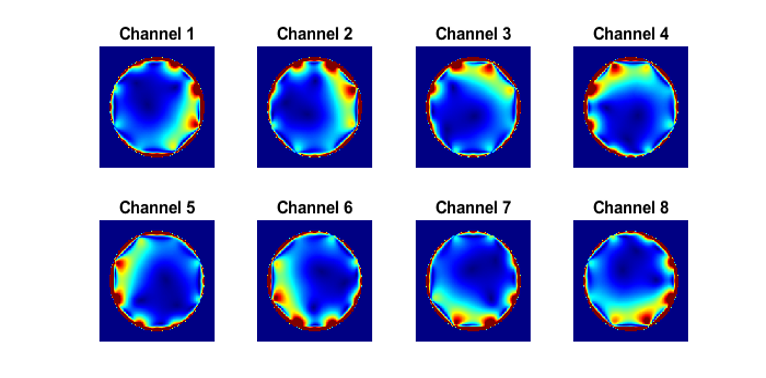
Figure 2, normalized 1W input B1+ magnitude profiles for the 8-channel dBC. B1+ maps are shown for the center slice of the dBC.
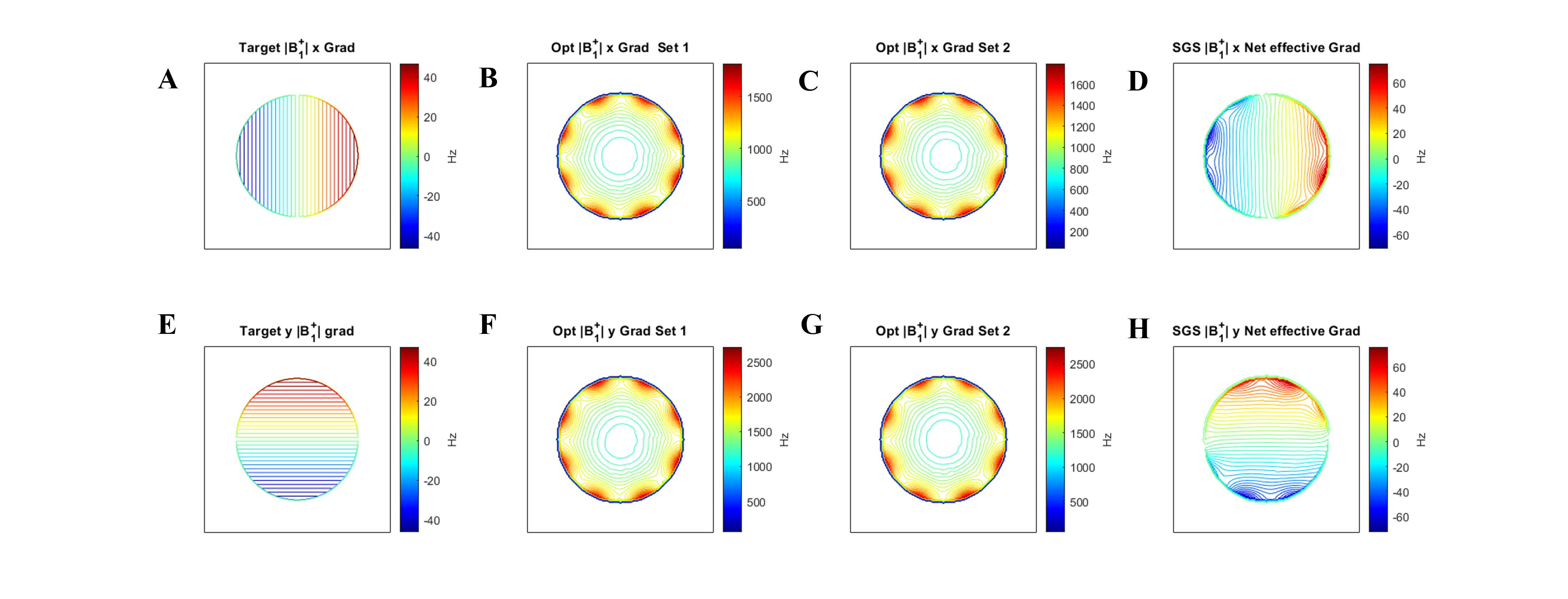
Figure 3, ML optimized RF gradients for SGS-FREE (A) ideal net x RF gradient magnitude, (B) and (C) ML optimized x RF gradient sets for SGS FREE, (D) generated net x SGS FREE effective gradient (w1max SGS Net x), (E) ideal net y RF gradient magnitude, (F) and (G) ML optimized y RF gradient sets for SGS FREE, (H) generated net y SGS FREE effective gradient (w1max SGS Net y). Note all maps show the inner 22.5 cm diameter imaging volume. Opt: optimized, Grad: Gradient
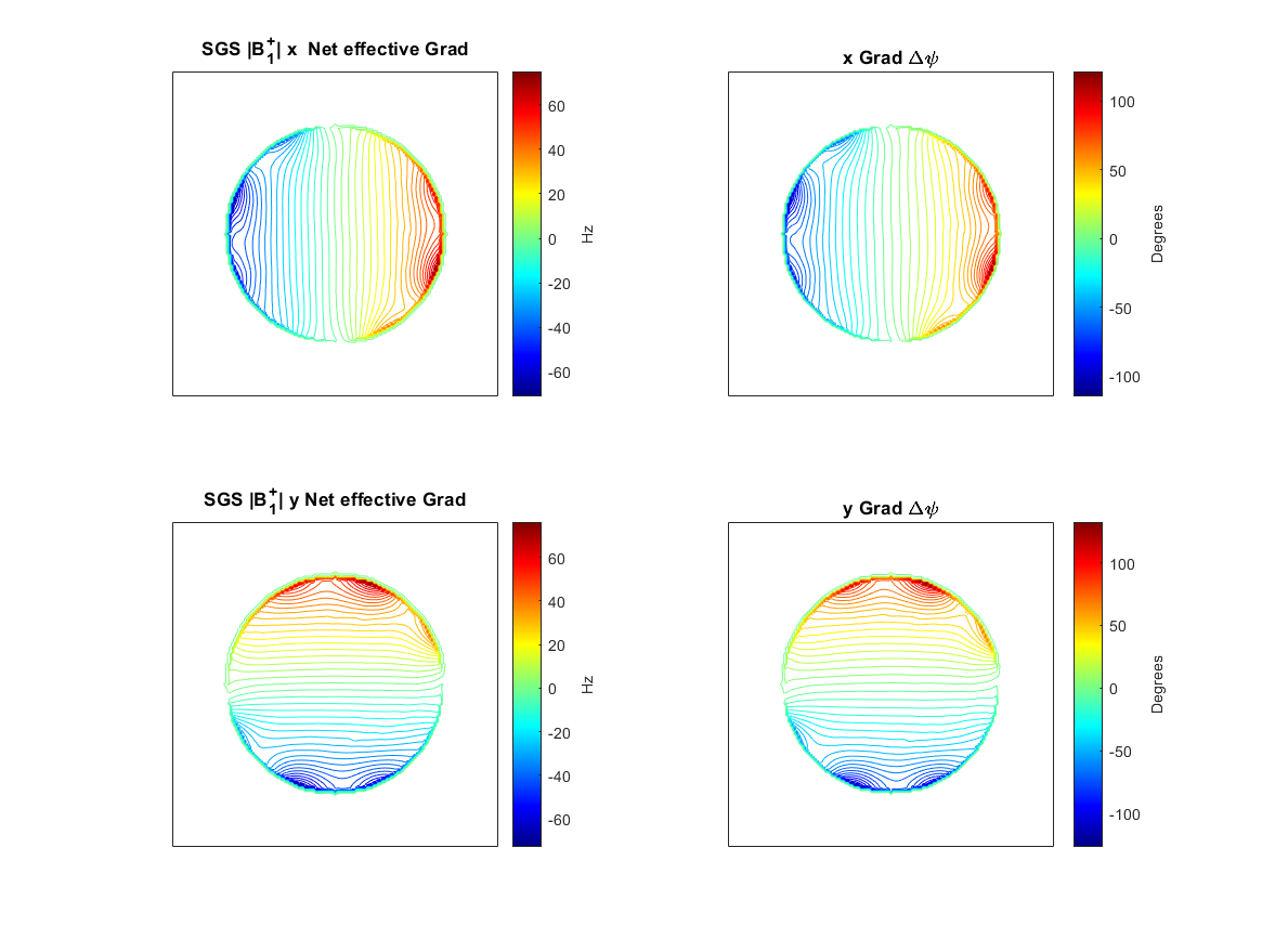
Figure 4, x and y SGS FREE net effective RF gradients compared with x and y Δψ(y) phase profiles generated. The proportionality between SGS FREE Net effective RF gradients and respective Δψ(y) phase maps demonstrates the SGS principle. Pulse parameters: AFP HS1 pulses, BWΩ = 2 KHz, Tp = 20ms, off-resonance = +/-500Hz. Grad: Gradient
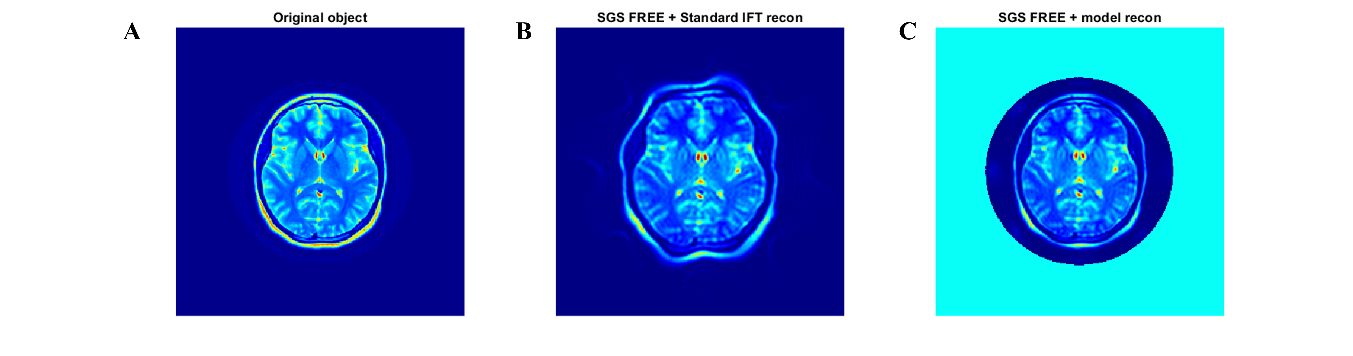
Figure 5, (A) original brain object, (B) 2D SGS FREE propagator analysis with standard IFT reconstruction, and (C) 2D SGS FREE propagator analysis with model-based reconstruction. 100 by 100 k-space cartesian sampling was used. A homogeneous receive field was assumed.
DOI: https://doi.org/10.58530/2023/0304