Synopsis

Keywords: Quantitative Imaging, Quantitative Susceptibility mapping

Conventional quantitative susceptibility mapping (QSM) reconstruction methods only provide voxel-averaged susceptibility value. We proposed a comprehensive complex signal model that describes the relationship between the 3D GRE signal and the contributions of opposing susceptibility to the frequency shift and $$$R_2^*$$$ relaxation. We used an iterative data fitting scheme to alternatively determine the sub-voxel susceptibilities and the voxel-wise proportionality coefficient between $$$R_2'$$$ and absolute susceptibility. Our experiments on in-vivo human brain data compared with histological staining images demonstrate that the proposed method provides more accurate results for quantifying brain iron and myelin than previous QSM separation methods.

Introduction

Advanced susceptibility imaging methods have been recently developed to distinguish the contributions of opposing susceptibility sources for QSM^1,2. The magnitude decay kernel, representing the proportionality constant between $$$R_2'$$$ and the absolute susceptibility, was considered spatial-invariant under the static dephasing regime³. However, this assumption is too ideal for modeling the real relationship between $$$R_2'$$$ and susceptibility in brain tissue. Here, we proposed a more comprehensive complex signal model that describes the relationship between the 3D GRE signal and the contributions of opposing susceptibility to the frequency shift and $$$R_2^*$$$ relaxation. We used an iterative data fitting scheme to alternatively determine the sub-voxel susceptibilities and the voxel-specific magnitude decay kernel between $$$R_2'$$$ and absolute susceptibility.

Methods

Improved QSM separation algorithm
In the magnetic field, the biological materials with susceptibility $$$\chi$$$ will induce inhomogeneities, resulting in frequency shift $$$\Delta f$$$ and $$$R_2' (=R_2^*-R_2)$$$ relaxation. Both $$$\Delta f$$$ and $$$R_2'$$$ can be formulated by paramagnetic susceptibility $$$\chi_{para}$$$ and diamagnetic susceptibility $$$\chi_{dia}$$$:
$$\left\{{\matrix{{\Delta f=D*\left({{\chi _{para}}+{\chi _{dia}}}\right)}\cr{{R_2'}=a\left({|{\chi_{para}}|+|{\chi_{dia}}|}\right)}\cr}}\right.\tag{1}$$
where $$$D$$$ is the dipole kernel and $$$*$$$ denotes the spatial convolution. $$$a$$$ is the magnitude decay kernel, representing the proportionality constant between $$$R_2'$$$ and the absolute susceptibility.
These inhomogeneities can be modeled using multi-echo GRE signal $$$S$$$:
$$S\left({T{E_j}}\right)={M_0}{e^{-\left({{R_2}+a|{\chi _{para}}\ \ |+a|{\chi_{dia}}\ |}\right)T{E_j}}}\cdot{e^{i\left\{ {{\phi_{res}}\ +2\pi f_{bg}\ TE_j+2\pi\gamma{B_0}\left[{D*\left({{\chi_{para}}\ \ +{\chi_{dia}}}\ \right)}\right]T{E_j}}\right\}}}\tag{2}$$
where $$$M_0$$$ is the extrapolated magnitude signal at echo time $$$(TE)$$$=0ms. $$$R_2$$$ relaxation can be obtained by an additional T2 mapping scan. $$$\phi_{res}$$$ is the time-independent initial phase. $$$\gamma$$$ is the gyromagnetic ratio and $$$2\pi {f_{bg}}{TE_j}$$$ denotes the background phase at $$$j^{\ th}$$$ echo times. The proposed method is eventually formulated as a two-step optimization. $$$M_0$$$ and $$$R_2^*$$$ can be firstly estimated using $$$N$$$ echo-time magnitude signals:
$$\mathop{\arg\min}\limits_{{M_0},\ R_2^*}\sum\limits_{j=1}^N{\left\|{\ln{M_j}-\left({\ln{M_0}-R_2^*T{E_j}}\right)}\right\|}_2^2\tag{3}$$
where $$${\left\|\cdot\right\|_2}$$$ denotes the $$$L2$$$ norm, and $$$M_j$$$ is the $$$j^{\ th}$$$ magnitude signal. The estimated $$$R_2^*$$$ was used in the next step to solve $$$\chi_{para}$$$ and $$$\chi_{dia}$$$:
$$\mathop{\arg\min}\limits_{{\chi_{para}}\ \ ,\ {\chi _{dia}}\ ,\ {\phi _{res}}}\left({\matrix{{{\lambda _1}\left\| {R_2^*-{R_2}-a\left({{\chi _{para}}-{\chi _{dia}}}\right)}\right\|_2^2}\cr{+\sum\limits_{j=1}^N{i\left\|{{\phi _{uw,\ T{E_j}}}-{\phi_{res}}-2\pi\left\{{{f_{bg}}+\gamma{B_0}\left[{D*\left({{\chi _{para}}+{\chi _{dia}}}\right)}\right]}\right\}T{E_j}}\right\|_2^2} }\cr{+{\lambda _2}\left\|{\chi-\left({{\chi_{para}}+{\chi _{dia}}}\right)}\right\|_2^2+{\lambda_3}\left({TV\left({{\chi_{para}}}\right)+TV\left({{\chi _{dia}}}\right)}\right)}\cr}}\right)\tag{4}$$
where $$$\phi _{uw,\ T{E_j}}$$$ is the unwrapped phase image, and $$$\chi$$$ is a pre-reconstructed QSM map. $$$TV(\cdot)$$$ is a 3D spatial total variation operator. $$$\lambda_1$$$, $$$\lambda_2$$$, and $$$\lambda_3$$$ are the regularization factors.
The proposed method regards the magnitude decay kernel as voxel-specific and resorts to an iterative algorithm to fit a voxel-wise $$$a$$$-map $$$(a')$$$:
$$a' = {{{R_2'}} \over {|{\chi _{para}}| + |{\chi _{dia}}|}}\tag{5}$$
The obtained parameter $$$a'$$$ is then plugged back into Eq. $$$(4)$$$ to recalculate $$$\chi_{para}$$$ and $$$\chi_{dia}$$$, then obtaining $$$a'$$$ following Eq. $$$(5)$$$ iteratively until convergence or the iterations reached 100.

Experiments
32 healthy human data were acquired at 3T. The 3D GRE scan parameters were: FOV=230×230×160mm³; matrix size=224×224×80; spatial resolution=1.03×1.03×2mm³; TR=40ms; TE₁/spacing/TE₇=2.4/4.3/28.2ms. The T2 mapping was acquired using 2D multi-echo spin echo (MSE) sequence with copied FOV from 3D GRE scan (TR=3864ms and TE₁/spacing/TE₅=16.1/16.1/80.5ms).
The $$$R_2$$$ map was fitted from MSE data using a mono-exponential function. The GRE phase data were unwrapped using a Laplacian-based phase unwrapping method⁴. The background phase and tissue phase were separated using V-SHARP method⁵. STAR-QSM⁶ was performed to pre-calculate QSM map. For comparison, a recent $$$\chi$$$-separation method¹ was used.

Results

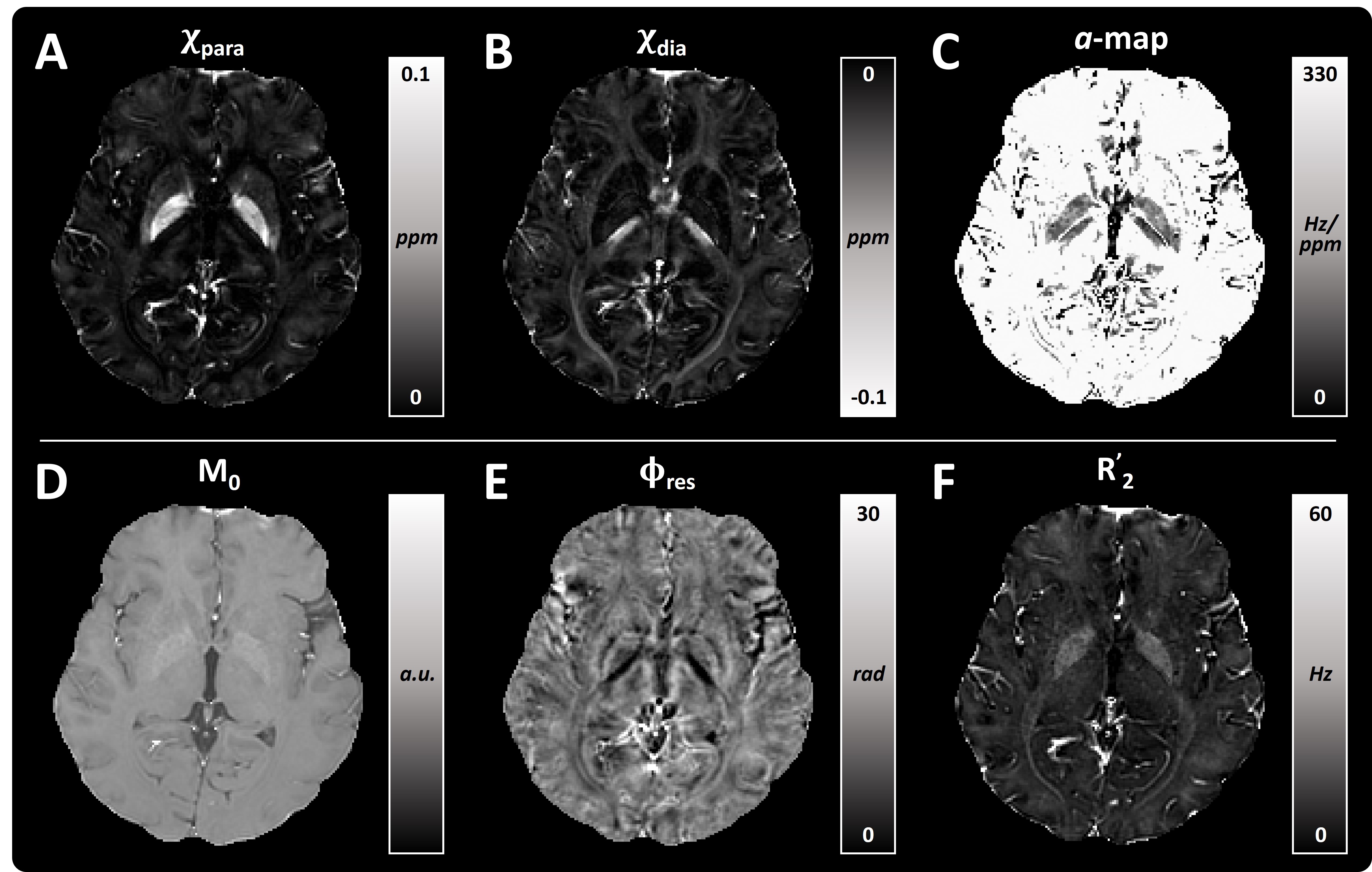
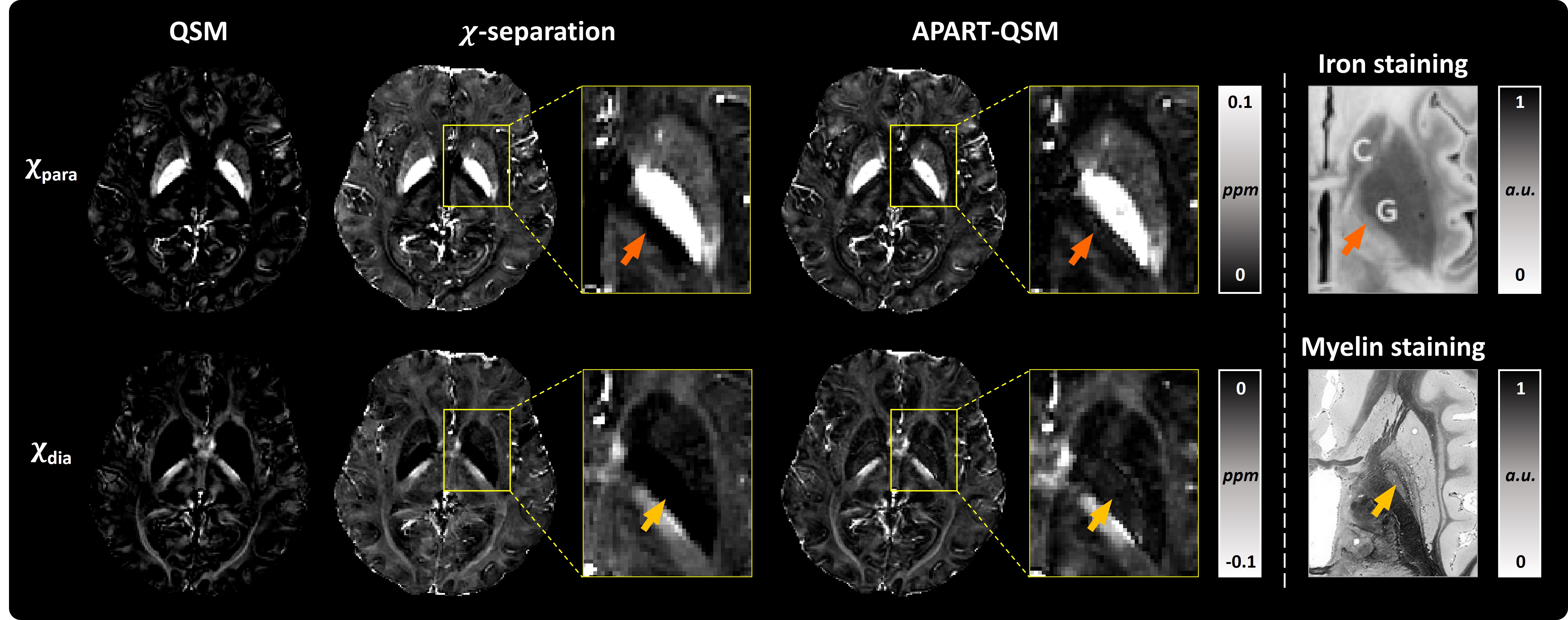
Fig. 1 shows the reconstructed maps of the healthy human data by the proposed method. $$$\chi_{para}$$$ map shows high positive values in deep gray matter (DGM) and blood vessels. $$$\chi_{dia}$$$ map reveals more negative susceptibility values in white matter. The magnitude decay kernels in the $$$a$$$-map decreased in the globus pallidus (GP) and some white matters. The $$$M_0$$$, $$$\phi_{res}$$$ and $$$R_2'$$$ maps are also shown in Fig. 1D, 1E and 1F.
Fig. 2 shows the comparison of the proposed method and $$$\chi$$$-separation’s results on the healthy subject with iron- and myelin-staining images from literature⁷ and website (https://brains.anatomy.msu.edu/). The $$$\chi_{para}$$$ map reconstructed from proposed method exhibits sparse positive susceptibility values in the posterior limb of the internal capsule (PLIC, orange arrows in the zoomed-in area), similar to the iron-staining image. However, the $$$\chi_{para}$$$ map from $$$\chi$$$-separation shows zero susceptibility values in PLIC. It is noted that the diamagnetic susceptibility values were clearly demonstrated in the GP by the proposed method’s $$$\chi_{dia}$$$ map, which is verified by the myelin staining (yellow arrows). In comparison, the $$$\chi_{dia}$$$ map reconstructed by $$$\chi$$$-separation shows barely diamagnetic susceptibility values in the GP.
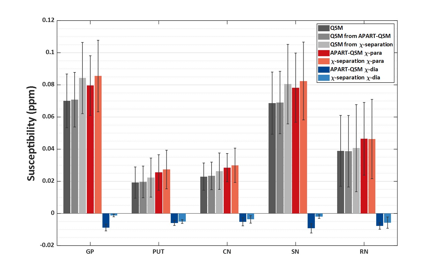
Quantitatively, Fig. 3 presents mean values of conventional QSM, $$$\chi_{para}$$$, $$$\chi_{dia}$$$ and composite QSM in five DGM nuclei averaged over 32 subjects. Both methods produce higher susceptibility values in these DGMs than conventional QSM. The proposed method shows more negative susceptibility values. The composite QSM by $$$\chi_{para}$$$ and $$$\chi_{dia}$$$ from proposed method shows more comparable mean values to the conventional QSM than that from $$$\chi$$$-separation.

Discussion and Conclusion

This study proposed a new magnetic susceptibility separation method, which utilizes a comprehensive complex model with an iterative data fitting algorithm to accurately separate intravoxel paramagnetic and diamagnetic susceptibility. Previous studies pre-determined a spatial-invariant magnitude decay kernel under the ideal static dephasing regime. Differently, our new method regards the magnitude decay kernel as voxel-specific, preventing the errors of the spatial-invariant kernel from propagating to the final QSM separation reconstruction. Thus, our method could be applied to quantifying the subtle magnetic susceptibility in brain tissue.

Acknowledgements

This study is supported by the National Natural Science Foundation of China (61901256, 91949120, 62071299).