Synopsis

Keywords: Machine Learning/Artificial Intelligence, Brain, Data Harmonization

For multi-site research in MR studies, a harmonization process is necessary. Due to the lack of paired dataset for harmonization, the unsupervised-based learning has been suggested. However, this method is susceptible to causing the error in anatomical information and performing well in the unseen domain. Thus, we suggest a deep neural network for multi-site harmonization based on MR signal physics with the paired traveling dataset. We implemented Quantitative Maps Generators and Denoising Network with the Bloch Equation module. We proved that using the Bloch Equation enhances the accuracy of harmonization.

Introduction

As multi-site research increases in MR field, the need for image harmonization is growing. However, MR image harmonization has been stuck in a holding pattern because of its sensitivity to experimental parameters and vendor dependency. Thus, cross-scanner harmonization is required¹. There were several studies^2-4 proposed unsupervised learning-based harmonization. However, the unsupervised method does not work well on unseen datasets. Furthermore, it is susceptible to causing unexpected artifacts or wrong anatomical details. In this study, we propose a neural network-based MR harmonization method utilizing Bloch Equation. The physics-based method reveals substantially improved harmonization results than other methods. Further, the proposed method can generate quantitative maps, such as T1 and M0 maps.

Methods

Dataset: All dataset was acquired from 3T scanners, and IRB approved.

1) Dataset of Quantitative Maps Generator: T1w images and T1map were acquired from 5 healthy controls using the MP2RAGE⁵ sequence. The M0map was estimated using Bloch Equation.

2) Dataset of Denoising Network: Traveling dataset was used. GE and Siemens T1w were acquired from 5 subjects using the inversion recovery sequence, whereas Philips T1w images were obtained from 4 healthy subjects with the fast spin echo sequence.

Preprocessing:
For the preprocessing, BET⁶, normalization, and N4-bais correction⁷ were applied. Each dataset for the Quantitative Maps Generator and Denoising Network was normalized as the following equation.
$$z_{target}=\frac{x_{source}-\mu_{target}}{\sigma_{target}}$$
,where $$$x_{source}$$$ is a T1w image of source scanner, $$$\mu_{target}$$$ and $$$\sigma_{target}$$$ are averaged mean and standard deviation of atarget scanner’s T1w images from the traveling dataset. $$$z_{target}$$$ is the normalized input T1w.

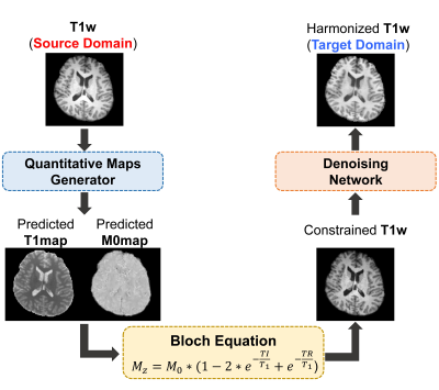
Bloch-informed Harmonization Network (BiHN): The overall schemes of BiHN process are shown in Fig. 1. BiHN consists of Quantitative Maps Generator, Bloch Equation module, and Denoising Network.

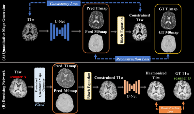
1) Training of the Quantitative Maps Generator: The 2D U-net⁸ based generator($$$U_{T1}$$$, $$$U_{M0}$$$) predicts the T1map and M0map from the acquired T1w image. (Fig.2 (A)). Adam⁹ optimizer was used for training the Quantitative Maps Generator. The learning rate was set to 0.001 and the max epoch was 500.

$$T1_{pred}=U_{T1}(T1w)$$
$$M0_{pred}=U_{M0}(T1w)$$
The constrained T1w (ConsT1w) was generated through the Bloch Equation with the predicted T1 and M0map assuming TI/TR=2400/4000ms.
$$ConsT1w=M0_{pred}*(1-2*e^{-\frac{TI}{T1_{pred}}}+e^{\frac{-TR}{T1_{pred}}})$$
The reconstruction loss was calculated between the predicted maps and ground truth.
$$ \mathcal{L}_{reconstruction} = \mathbb{E}[(M0_{GT}-M0_{pred})^2]+\mathbb{E}[(T1_{GT}-T1_{pred})^2]$$
The consistency loss was calculated between ConsT1w and input T1w. This loss constrained the generator to preserve the anatomical detail.
$$ \mathcal{L}_{consistency} = \mathbb{E}[(ConsT1w-T1w_{input})^2]$$
The total loss is defined as the following.
$$ \mathcal{L}_{total} =\lambda_{reconstruction}\mathcal{L}_{reconstruction} + \lambda_{consistency}\mathcal{L}_{consistency}$$
,where $$$\lambda_{reconstruction}$$$, $$$\lambda_{consistency}$$$ were set to 1.

2) Training of the Denoising Network: The Denoising Network was trained for three harmonization pairs, such as (i) GE↔Siemens, (ii) Siemens↔Philips, and (iii) Philips↔GE. Total 6 of 2D U-net ($$$U_{soruce\leftrightarrow target}$$$) were trained with the paired traveling dataset(Fig.2 (B)).

2)-(a) Pre-trained Quantitative Maps Generator: The generator predicts T1 and M0map from the traveling dataset as fixed.

2)-(b) Bloch Equation module: The equation is defined as a T1w for a target scanner.
$$ConsT1w=M0_{pred}*(1-2*e^{\frac{-TI}{T1_{pred}}}+e^{\frac{-TR}{T1_{pred}}})$$
,where TI and TR were set to scan parameters for each target scanner. For Siemens, TI/TR= 1000/2400ms. For GE, TI/TR=1600/2400ms. For Philips, the same parameters used in Siemens were applied.

2)-(c) Denoising Network: This step removes residual noise in the constrained T1w. Adam optimizer was also used for training of the Denoising Network. The learning rate was set to 0.001 and the max epoch was 100.
$$\hat{T}1w = U_{soruce\leftrightarrow target}(ConsT1w)$$
,where $$$\hat{T}1w$$$ is the harmonized T1w.
The reconstruction loss minimized the difference between the constrained T1w and the ground truth of the target scanner’s T1w.
$$\mathcal{L}_{reconstruction} = \mathbb{E}[(\hat{T}1w-T1w)^2]$$

Results

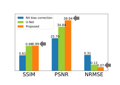
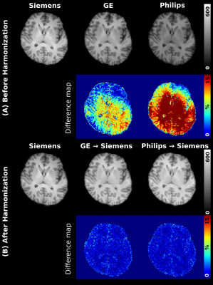
We compared the harmonization result from the proposed method to that from N4 bias correction, which is not a deep learning-based method. U-net without physics information was also compared. Figure 3 shows the averaged evaluation scores. In SSIM, Unet and the proposed method show similarly high scores of 0.98 and 0.99. PSNR was increased to 14.24dB than N4 bias correction, to 5.1 dB than Unet. The proposed method has also the lowest NRMSE. Figure 4 shows comparison results from before and after harmonization using BiHN. When compared difference maps, the error rate between Siemens T1w and harmonized T1w images were significantly decreased.

Conclusion & Discussion

In this study, we demonstrated that the Bloch Equation improved the harmonization accuracy. Furthermore, BiHN can generate T1 and M0maps while harmonizing T1w. Also, the Denoising Network does not require long training time. Therefore, through this study, we suggest the possibility to construct a synthesized T1w dataset using various scan parameters. Additionally, because BiHN was trained using the paired dataset, we solved inherent problem in deep neural network-based harmonization studies, such as generating inaccurate tissues or unexpected noises. Our ultimate goal is to suggest a standardized contrast that is not susceptible to scanner effects.

Acknowledgements

This work was supported by the MSIT (Ministry of Science, ICT), Korea, under the High-Potential Individuals Global Training Program (2021-0-01553), supervised by the IITP (Institute for Information & Communications Technology Planning & Evaluation), and the National Research Foundation of Korea (NRF) grant, funded by the Korean government (MSIT) (NRF-2020R1A2C4001623).

References

1. Crombé, Amandine, Michèle Kind, David Fadli, François Le Loarer, Antoine Italiano, Xavier Buy, and Olivier Saut. "Intensity harmonization techniques influence radiomics features and radiomics-based predictions in sarcoma patients." Scientific reports 10, no. 1 (2020): 1-13.

2. Liu, Mengting, Piyush Maiti, Sophia Thomopoulos, Alyssa Zhu, Yaqiong Chai, Hosung Kim, and Neda Jahanshad. "Style transfer using generative adversarial networks for multi-site mri harmonization." In International Conference on Medical Image Computing and Computer-Assisted Intervention, pp. 313-322. Springer, Cham, 2021.

3. Zuo, Lianrui, Blake E. Dewey, Yihao Liu, Yufan He, Scott D. Newsome, Ellen M. Mowry, Susan M. Resnick, Jerry L. Prince, and Aaron Carass. "Unsupervised MR harmonization by learning disentangled representations using information bottleneck theory." NeuroImage 243 (2021): 118569.

4. Guan, Hao, Yunbi Liu, Erkun Yang, Pew-Thian Yap, Dinggang Shen, and Mingxia Liu. "Multi-site MRI harmonization via attention-guided deep domain adaptation for brain disorder identification." Medical Image Analysis 71 (2021): 102076.

5. Marques, José P., Tobias Kober, Gunnar Krueger, Wietske van der Zwaag, Pierre-François Van de Moortele, and Rolf Gruetter. "MP2RAGE, a self bias-field corrected sequence for improved segmentation and T1-mapping at high field." Neuroimage 49, no. 2 (2010): 1271-1281.

6. S.M. Smith. Fast robust automated brain extraction. Human Brain Mapping, 17(3):143-155, November 2002.

7. Tustison, Nicholas J., Brian B. Avants, Philip A. Cook, Yuanjie Zheng, Alexander Egan, Paul A. Yushkevich, and James C. Gee. "N4ITK: improved N3 bias correction." IEEE transactions on medical imaging 29, no. 6 (2010): 1310-1320.

8. Ronneberger, Olaf, Philipp Fischer, and Thomas Brox. "U-net: Convolutional networks for biomedical image segmentation." In International Conference on Medical image computing and computer-assisted intervention, pp. 234-241. Springer, Cham, 2015.

9. Kingma, Diederik P., and Jimmy Ba. "Adam: A method for stochastic optimization." arXiv preprint arXiv:1412.6980 (2014).