0163
MR image super-resolution via a variational diffusion model1University of Queensland, Brisbane, Australia
Synopsis
Keywords: Machine Learning/Artificial Intelligence, Image Reconstruction, MRI, diffusion models
High-resolution MR images are advantageous for medical diagnosis. However, they may require longer scan time and more powerful hardware. Significant effort has been made to carry out super-resolution methods to synthesize higher-resolution MR images from lower-resolution acquisitions using deep learning approaches. However, most current methods are biased. In this work, we propose a new super-resolution method based on the state-of-the-art generative model (i.e., variational diffusion model), using the lower-resolution K-space measurements as a condition for guiding the super-resolution process. This unsupervised approach achieved high performance for reconstructing MR images from arbitrary lower resolutions without retraining the model.Introduction
The low resolution of medical images hampers the medical diagnosis. Significant effort has been made to carry out new methods for improving image resolution using deep learning. Recently, Chitwan Saharia et.al4 proposed an Image Super-Resolution based on diffusion models and achieved high-fidelity images with high resolutions. However, this model is not applicable in real-world super-resolution tasks due to its bias caused by mode dropping4. We propose a new Super-Resolution method conditioned on low-resolution MRI acquisitions through a generative model in this work.Methods
In this work, we first train a VDM2 model with high-resolution brain MR images to estimate the distribution of these high-resolution images. We then use this modelled distribution of high-resolution images as a data-driven prior to assist image-super resolution task from MR measurements of lower resolution. Specifically, during the sampling process of VDM, we synthesize higher-resolution images by applying the low-resolution k-space measurement as a guide for the generation process inspired by Song et al.3.VDM
The Variational Diffusion Model2 (VDM) is an improved version of the original Denoising Diffusion Probabilistic models1(DDPM). It uses signal-to-noise ratio (SNR) to represent the noise schedules of the diffusion process. This SNR not only simplified the mathematical formula but also help to improve the model's architecture, leading to state-of-the-art likelihoods on image density. In the implementation of VDM, this model incorporates Fourier Features techniques, which further improved the likelihood of image density.
The diffusion process can be described as a Markovian process: $$q(\boldsymbol{x}_{t}|\boldsymbol{x}_{t-1})=\mathcal{N}(\boldsymbol{x}_{t};\alpha_{t}\boldsymbol{x}_{t-1},\beta_{t}^{2}\boldsymbol{I})$$
Here we let $$$\alpha_t=\sqrt{1-\beta_t^2}$$$, and this is called the variance-preserving diffusion process.
In VDM, we define $$$\text{SNR}(t)=\alpha_t^2 / \beta_t^2 $$$. Let $$$\text{SNR}(t)=\exp(-\gamma_\boldsymbol{\phi}(t))$$$, and let $$$\gamma_\boldsymbol{\phi}(t)$$$ be a monotonic neural network with parameters $$$\boldsymbol{\phi}$$$ to learn the noise schedule. This is different from other implementations of diffusion models, which fix the noise schedule as hyperparameters.
We optimize the model using the variational lower bound, and the objective function has three parts, the prior loss, reconstruction loss, and diffusion loss. The first two loss terms are similar to the variational autoencoder (VAE). The diffusion loss can be simplified as:$$\mathcal{L}_{T}(\boldsymbol{x})=\dfrac{T}{2}\mathbb{E}_{\epsilon\sim\mathcal{N}(\boldsymbol{0},\boldsymbol{I}),t\sim U\{1,T\}}\left[(\exp(\gamma_{\boldsymbol{\phi}}(t)-\gamma_{\boldsymbol{\phi}}(s))-1)\|\boldsymbol{\epsilon}-\boldsymbol{\epsilon}_{\boldsymbol{\theta}}(\boldsymbol{x}_{t};t)\|_{2}^{2}\right]$$where $$$t>s$$$ and $$$\boldsymbol{x}_{t}=\text{sigmoid}(-\gamma_{\boldsymbol{\phi}}(t))\boldsymbol{x}_{0}+\text{sigmoid}(\gamma_{\boldsymbol{\phi}}(t))\boldsymbol{\epsilon}$$$ and $$$\boldsymbol{\epsilon}_{\boldsymbol{\theta}}(\boldsymbol{x}_{t})$$$ represents the neural network model that can predict noise at each step. Once we trained the model $$$\boldsymbol{\epsilon}_{\boldsymbol{\theta}}(\boldsymbol{x}_{t};t)$$$, we can use it to remove noise from images gradually, and finally get the denoised brain MR images. Each sampling step can be written as:$$\boldsymbol{x}_{t-1}=a(\boldsymbol{x}_{t}-b\boldsymbol{\epsilon}_{\boldsymbol{\theta}}(\boldsymbol{x}_{t};t))+c\boldsymbol{\epsilon}$$where $$$a,b,c$$$ are depend on $$$\gamma_{\boldsymbol{\phi}}$$$ only.
K-space method
Here we use k-space measurement as guidance to perform the super-resolution task. Let $$$\boldsymbol{F}$$$ represent the Fourier transform from image space to k-space, and $$$\boldsymbol{F}^{-1}$$$ represents the inverse. The low-resolution k-space measurement $$$\hat{\boldsymbol{y}}_0$$$ can be modelled by the high-resolution image $$$\boldsymbol{x}_0$$$ transformed into high-resolution kspace, cropped out only the low-resolution central region of k-space:$$\hat{\boldsymbol{y}}_0=\mathcal{p}^{-1}(\boldsymbol{\Lambda})\boldsymbol{F}\boldsymbol{x}_0+\boldsymbol{\epsilon}$$where $$$\boldsymbol{\epsilon}\sim\mathcal{N}(\boldsymbol{0},\boldsymbol{I})$$$ represents the Gaussian noise during signal acquisition, $$$\boldsymbol{\Lambda}$$$ represents the downsampling mask, and $$$\mathcal{p}^{-1}(\boldsymbol{\Lambda})$$$ represents cropping out only the centre of the full kspace. Similarly, we can perturb the low-resolution k-space measurement by $$$\hat{\boldsymbol{y}}_t=\sqrt{1-\beta_{t}}\hat{\boldsymbol{y}}_0+\sqrt{\beta_{t}}\mathcal{P}^{-1}(\boldsymbol{\Lambda})\boldsymbol{F}\boldsymbol{\epsilon}$$$ at each sampling step, and then add an extra step to use the perturbed $$$\hat{\boldsymbol{y}}_t$$$ to guide image generation process:$$\boldsymbol{x}_{t}'=\boldsymbol{F}^{-1}\underset{\text{1}}{[\underbrace{\lambda\mathcal{p}(\boldsymbol{\Lambda})\hat{\boldsymbol{y}}_{t}+(1-\lambda)\boldsymbol{\Lambda}\boldsymbol{F}\boldsymbol{x}_{t}}}+\underset{2}{\underbrace{(\boldsymbol{I}-\boldsymbol{\Lambda})\boldsymbol{F}\boldsymbol{x}_{t}}}]$$where $$$\mathcal{p}(\cdot)$$$ is padding operation, the reverse of cropping out. In the formula, part 1 describes the mixture of $$$\mathcal{p}(\boldsymbol{\Lambda})\hat{\boldsymbol{y}}_t$$$ and $$$\boldsymbol{\Lambda}\boldsymbol{F}\boldsymbol{x}_t$$$ on the measured central k-space region with λ as the mixture weight, balancing data fidelity and image prior. Part 2 is the generation of the unmeasured outer k-space region from the trained diffusion model. The updated $$$\boldsymbol{x}_{t}'$$$ will be fed forward to the next denoising step.
Experiments
We trained the diffusion model using a brain MRI dataset with 130k gradient-echo magnitude images (2D axial, 8 echoes from 4 ms to 30 ms) from 300 subjects. Each image is resized to 128x128 (2mm in-plane resolution) to fit in GPU memory. Due to the hardware limitation, we demonstrate the idea by training a model with 128x128 (i.e., 2mm isotropic resolution) images as the reference high-resolution images. We then retrospectively downsampled the testing data further to lower resolutions of matrice sizes 32x32 and 64x64. We implemented this diffusion model with a U-Net of depth 32, and trained this model in A100 GPU with 40G memory for 2 days. The number of steps was set to 1000. It takes about 2 mins to sample a batch of 4 images on the same GPU.Results
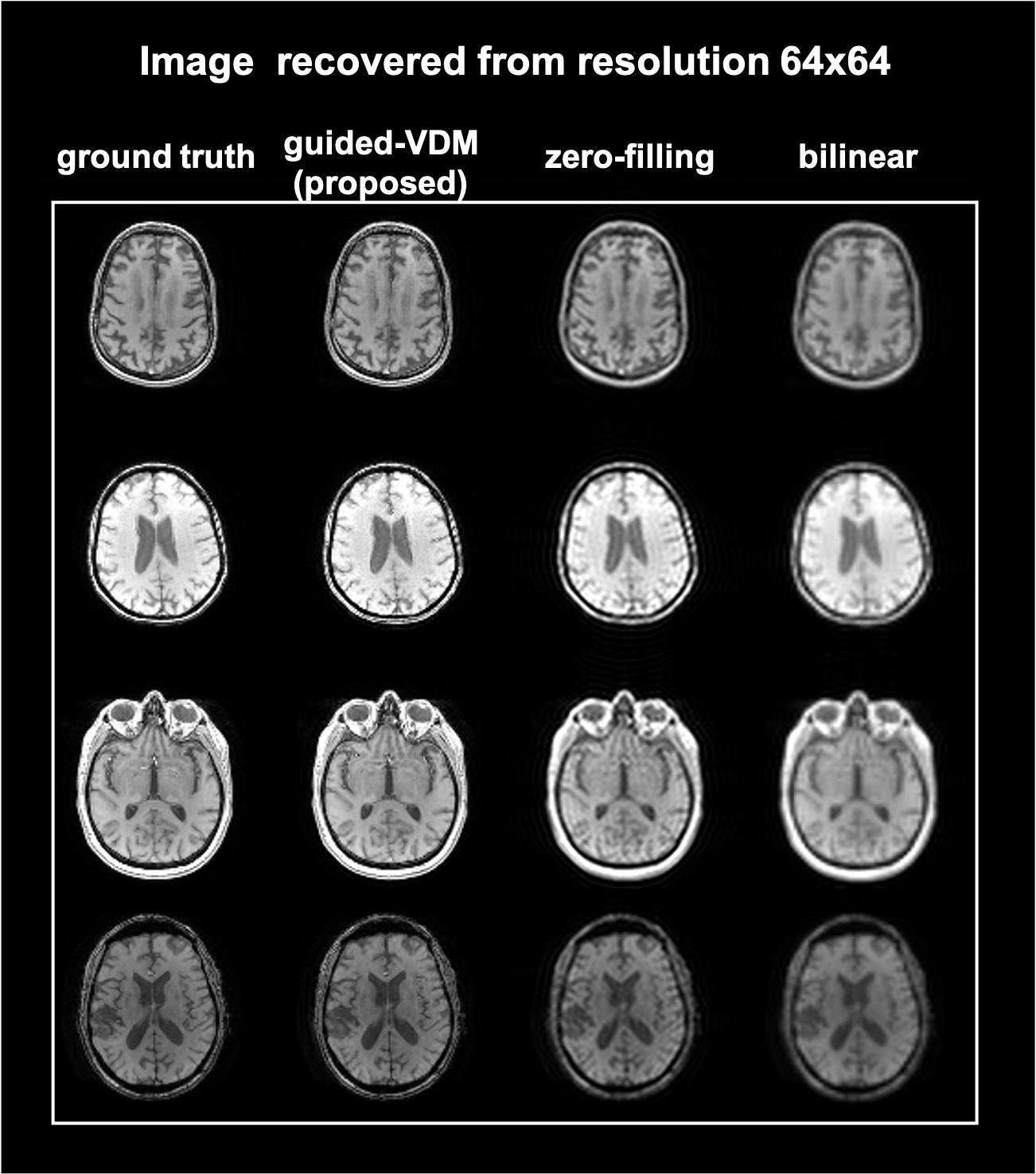
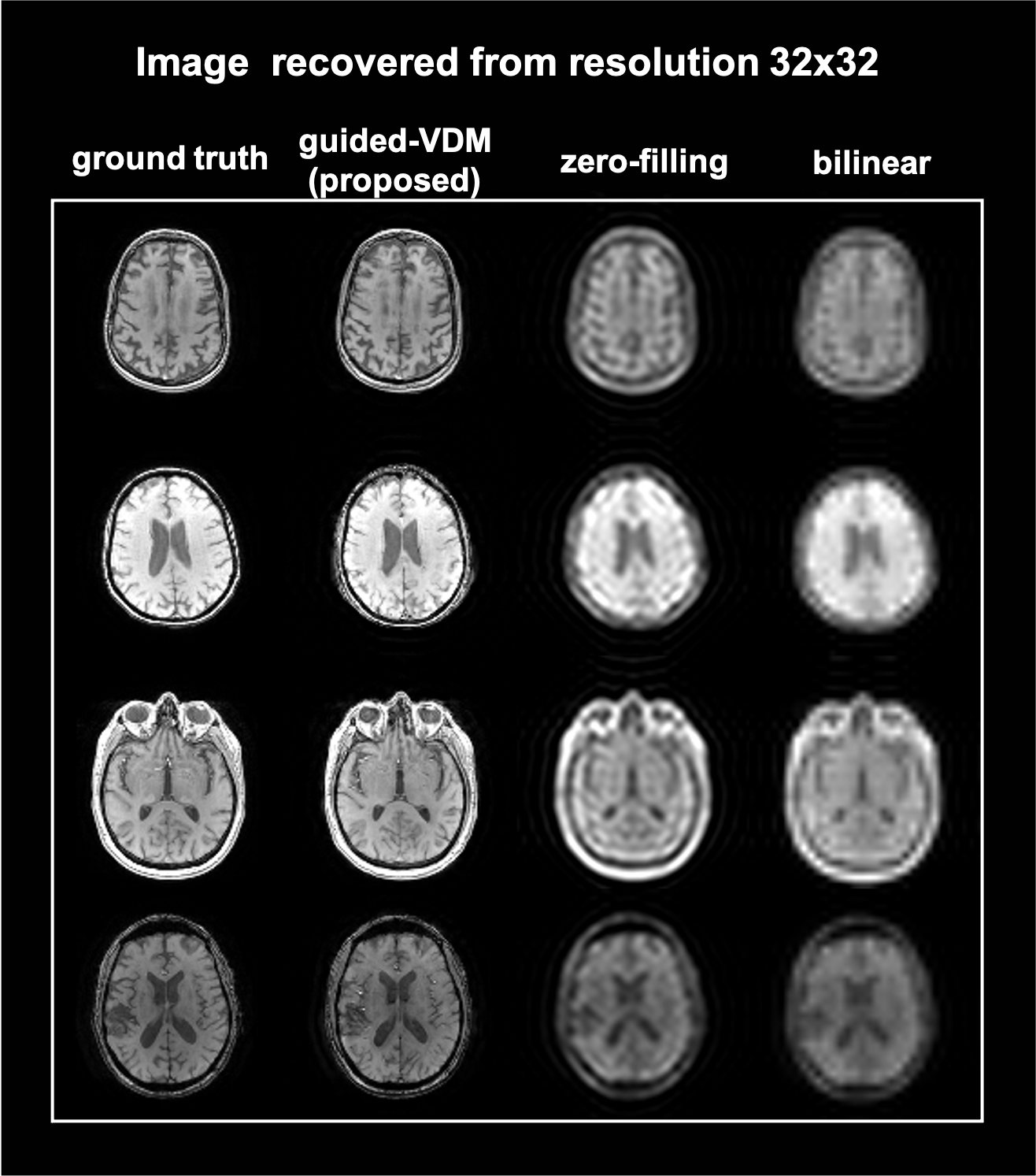
Figure 1(a) illustrates the forward and reverse processes of VDM. (b) shows the correction step during the sampling process.Super-resolution results from lower-resolution of matrix sizes 64*64 and 32*32 to higher-resolution of 128*128 are shown in Fig.2 and Fig.3 respectively. The proposed guided-VDM method generated significantly higher-quality images as compared to zero-filling and bilinear-interpolation methods.
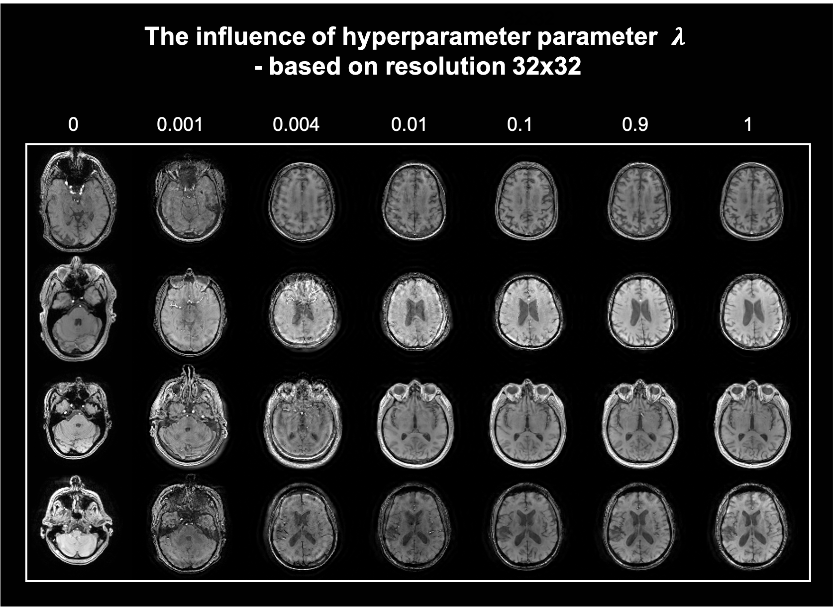
Fig. 4 demonstrates the k-space guidance effect by different weighting factors λ, which indicates the influence of the low-resolution K-space measurement. The whole generative process can be correctly guided even with a small λ.
Conclusion
We have proposed a new super-resolution method conditioned on low-resolution MRI k-space measurements. This method is based on a state-of-the-art diffusion model with conditional generation and can synthesize high-quality MRI images from arbitrary low-resolution MRI acquisitions without retraining the model.Acknowledgements
HS received funding from Australian Research Council (DE210101297).References
1. Ho J, Jain A, Abbeel P. Denoising diffusion probabilistic models. Advances in Neural Information Processing Systems. 2020;33:6840-51.
2. Kingma D, Salimans T, Poole B, Ho J. Variational diffusion models. Advances in neural information processing systems. 2021 Dec 6;34:21696-707.
3. Song Y, Shen L, Xing L, Ermon S. Solving inverse problems in medical imaging with score-based generative models. arXiv preprint arXiv:2111.08005. 2021 Nov 15.
4. Saharia C, Ho J, Chan W, Salimans T, Fleet DJ, Norouzi M. Image super-resolution via iterative refinement. IEEE Transactions on Pattern Analysis and Machine Intelligence. 2022 Sep 12.
Figures
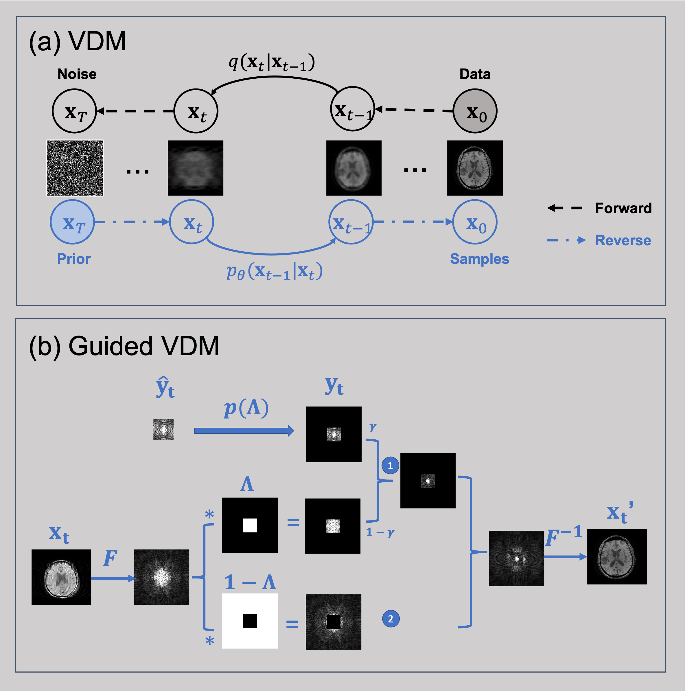
Fig. 1(a) illustrates the forward and reverse processes of VDM (b) shows the correction step during the sampling process by incorporating low-resolution k-space measurement as data fidelity.