0155
Adaptive convolution for including a-priori information in deep learning models for quantitative susceptibility mapping
Simon Graf1, Nora Küchler1, Walter Wohlgemuth1, and Andreas Deistung1
1University Hospital Halle (Saale), Halle (Saale), Germany
1University Hospital Halle (Saale), Halle (Saale), Germany
Synopsis
Keywords: Machine Learning/Artificial Intelligence, Quantitative Susceptibility mapping
Deep learning models used for solving dipole inversion of quantitative susceptibility mapping typically lack an integration of a-priori information. We show for the first time that information of voxel-size and field-of-view orientation with respect to B0 can be incorporated into network models by deploying adaptive convolution. Various network models were trained for 170 epochs to solve dipole inversion on synthetic data with arbitrary orientation and voxel-sizes. Adaptive convolution models outperform conventional models in computing susceptibility maps from arbitrarily oriented field distributions with anisotropic voxel sizes and allows a reduction of training time.Introduction
While convolutional neural networks (CNNs) have been used extensively to solve the inverse problem to convert the magnetic field to magnetic susceptibility in quantitative susceptibility mapping (QSM) 1,2, limitations regarding their applicability in clinical settings still remain. So far, current QSM network models do not leverage known a-priori information. Known aspects like the voxel aspect ratio (VAR) or the orientation of the field-of-view (FOV) with respect to B0 are generally not considered. Recently, incorporation of side information in network models was proposed in crowd counting with cameras3. Motivated by this approach, we demonstrate for the first time the use of adaptive convolution (AC) to incorporate a-priori information into deep learning models for QSM dipole inversion.Theory
AC identifies changes in the input associated with the presented side information and correlates these with network parameters. When the convolutional filter weights are considered as points on a low-dimensional manifold in the high-dimensional filter weight space, the weights move on the manifold (Fig. 1). Hence, the convolution filter weights change adaptively as a function of the side information and, thus, the network is expected to learn the relationship between the susceptibility map and B-field distribution more easily. AC-layers are built from feed-forward networks to model the filter manifold (Fig. 2). The filter manifold network (FMN) computes convolutional filter weights and bias of the adaptive convolution layer. Overall, by giving side information to the AC layer, the most suitable filter weights are chosen to compute output feature maps.Methods
A U-Net4 with Octave Convolution5 was trained to predict the 3D susceptibility map from the same-sized magnetic field distribution (Fig. 3). The network architecture of all models was five layers deep with 16 initial channels. Different placements of the AC-layer in the U-Net (Fig. 3), at the first block (First) and the first encoding block (Enc1), were tested. 1000 synthetic non-anatomical susceptibility maps (320x320x320) compromising randomly distributed shapes with susceptibilities from a Gaussian distribution (µ=0, σ=0.25) served as training data. The z-component of the voxels-size was drawn from the uniform distribution [1, 6] while the x- and y-component remained constant at one. Different FOV-orientations were simulated by randomly rotating B0=[0,0,1]T around the x-, y- and z-axis. The x- and y-values were drawn from the Gaussian distribution (µ=0, σ=11) and the z-values from (µ=0, σ=15). Variations in voxel-size and B0 occurred with probability 0.8, ensuring standard parameters in the training data. The B-field distribution was obtained via fast forward convolution in k-space6. 64 patches of dimension 64x64x64 were randomly extracted from these datasets at each iteration for network training. All models were trained with the Adam optimizer7 for 170 epochs and learning rate of 0.001. The mean-squared-error served as loss metric and training was performed on an NVIDIA QUADRO RTX 6000. Validation was performed after each epoch on 100 validation datasets. The network models were evaluated on synthetic data corresponding to the training dataset to increase comparability of results and assessment.Results
NRMSE, SSIM and visual assessment metrics (Fig. 4) show that placing the AC-layer at the first encoding block (Enc1) leads to susceptibility maps with higher similarity to the ground truth. Substantial differences to the ground truth are visible for the susceptibility map computed by the conventional model (Fig. 4). The computed susceptibility map lacks on sharp edges, well-resolved shapes, appears generally blurred and a Moiré pattern is present. The metrics of the adaptive model (Enc1) show its superiority over the conventional model.Discussion
The parameters for the FMN were chosen based on recommendations for crowd counting3. It was assumed that a similar number of layers and parameters are required to obtain FMNs that can comprehensively learn the relationship between the side information and the associated changes in the image -the filter manifold- and are consequently able to adapt the kernel parameters. The AC-layer must be placed at a level in the network where changes in the image associated with the side information are most pronounced. The results show that this is the case by placing the AC in the first encoding block (First) as indicated by sharp edges in the activation maps (Fig. 3B). Consequently, the FMN can more easily correlate the side information with changes in the feature maps. The conventional model without AC cannot compute valuable susceptibility maps from arbitrary-orientation magnetic field distributions sampled with anisotropic voxels and would require considerably more training epochs. This implies that less data and training time is required for training AC network models. Remaining differences between reconstructed and ground truth susceptibilities can be reduced with more training epochs. Standard QSM dipole inversion algorithms make use of additional parameters to find optimal solutions. Similarly, we believe that providing a-priori information acts as constraint for parameter optimization, guiding the network towards valid solutions. In future studies, we will investigate different ways to add side information to the network, optimize the FMN and integrate AC in different network architectures.Conclusion
Side information can be incorporated in AC network models to solve the ill-posed QSM dipole inversion. Network models including AC perform superior on datasets with arbitrary orientations and anisotropic voxel-size and offer the possibility to reduce training time.Acknowledgements
This project was supported by the European Regional Fund (ERDF - IP* 1b, ZS/2021/06/158189).
References
- Yoon J, Gong E, Chatnuntawech I. (2018). Quantitative susceptibility mapping using deep neural network: QSMnet. Neuroimage. https://doi.org/10.1016/j.neuroimage.2018.06.030
- Bollmann S, Rasmussen KGB, Kristensen M, etal. (2019). DeepQSM - using deep learning to solve the dipole inversion for quantitative susceptibility mapping. Neuroimage. https://doi.org/10.1016/j.neuroimage.2019.03.060
- Kang D, Dhar D, Chan AB. (2020). Incorporating Side Information by Adaptive Convolution. Int. J. Comput. Vision. https://doi.org/10.1007/s11263-020-01345-8
- Ronneberger O, Fischer P, Brox T. (2015). U-Net: Convolutional Networks for Biomedical Image Segmentation. Medical Image Computing and Computer-Assisted Intervention – MICCAI 2015. https://doi.org/10.1007/978-3-319-24574-4_28
- Gao Y, Zhu X, Moffat BA, et al. (2021). xQSM: quantitative susceptibility mapping with octave convolutional and noise-regularized neural networks. NMR in Biomedicine. https://doi.org/10.1002/nbm.4461
- Marques P, Bowtell R. (2005). Application of a Fourier‐based method for rapid calculation of field inhomogeneity due to spatial variation of magnetic susceptibility. https://doi.org/10.1002/cmr.b.20034
- Kingma, DP, Ba J. (2014). Adam: A Method for Stochastic Optimization. https://doi.org/10.48550/arxiv.1412.6980
Figures
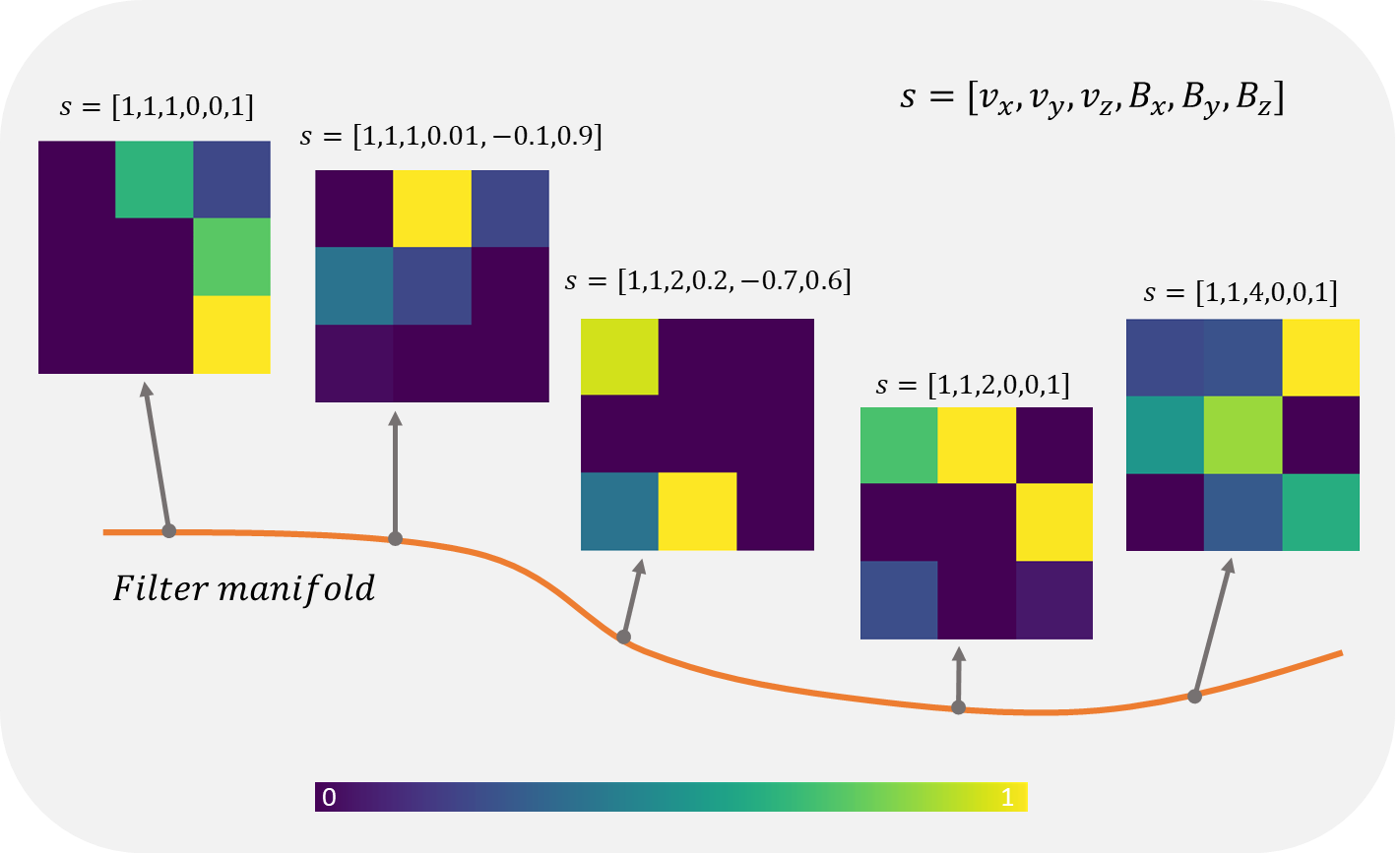
Figure 1: The side information array s, containing the voxel-size v and the B0-vector, is modeled by the filter manifold network (FMN) to a low-dimensional filter manifold in the high-dimensional filter weight space. Depending on the given side information, the convolutional filter weights (convolution kernel), depicted by the color-coded squares, change their values. Hence, the FMN selects the most suitable convolution filter values to compute the output feature maps.
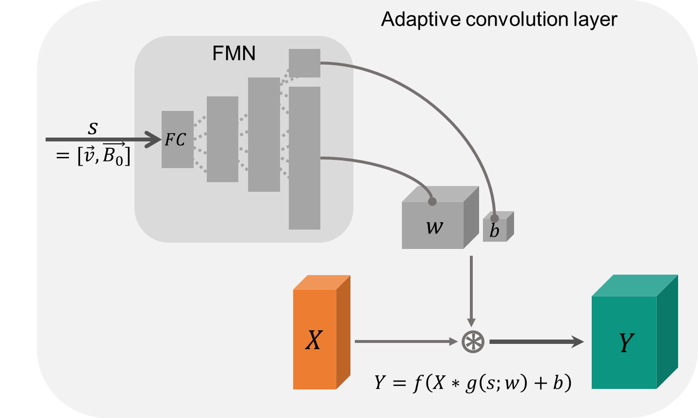
Figure 2: The adaptive convolution layer (light grey) consists of the filter manifold network (FMN) with four fully connected (FC) layers (dark grey bars) utilizing the side information s (voxel-size and B0) to compute the filter weights w and the bias b. After reshaping into suitable tensors, the adaptive kernel g is convolved with the input feature map X producing the output feature map Y. f denotes the ReLU activation function.
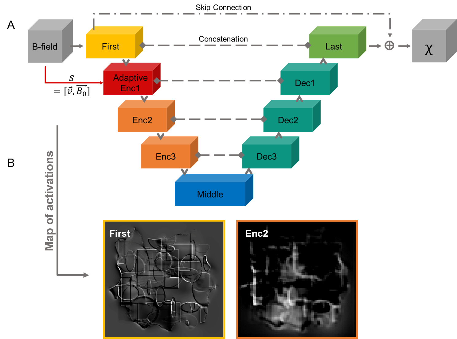
Figure 3: Depiction of the U-Net with adaptive convolution placed at the first encoding block (A). The network gets magnetic field distributions and computes susceptibility maps. Side information is directly propagated to the adaptive layer. Activation maps (B) computed without the adaptive layer of the first block (First) and second encoding block (Enc2) are shown, emphasizing that edges are extracted by the first block (First) and higher-level features by deeper encoding blocks (e.g. Enc2).
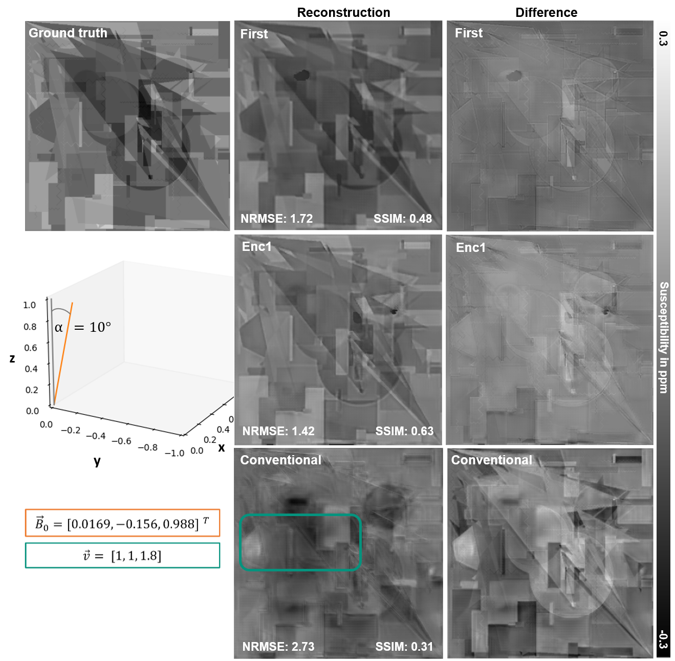
Figure 4: The reconstructed susceptibility maps (voxel-size: 1x1x1.8mm³) with the adaptive layer placed at the first block (First) and first encoding block (Enc1) and the conventional model are shown. The turquoise rectangle labels a Moiré pattern. The susceptibility maps of the adaptive models resemble the ground truth map with Enc1 achieving highest visual and metric similarity. Substantial differences to the ground truth are present in the susceptibility map of the conventional model.
DOI: https://doi.org/10.58530/2023/0155