0107
Adaptive Magnetic Resonance1Chemical and Biological Physics, Weizmann Institute of Science, Rehovot, Israel, 2Siemens Healthcare Ltd., Rosh Haayeen, Israel
Synopsis
Keywords: Hybrid & Novel Systems Technology, Pulse Sequence Design, Accelerating data acquisition
We present a completely general framework for adaptively changing the radiofrequency pulses and delays in real time in response to incoming data from the subject within the scanner. This "personalized-radiology" framework is shown to increase the precision of T2 estimation for n-acetyl-aspartate in-vivo by a factor of 1.7, and accelerate its acquisition 2.5-fold.
Introduction
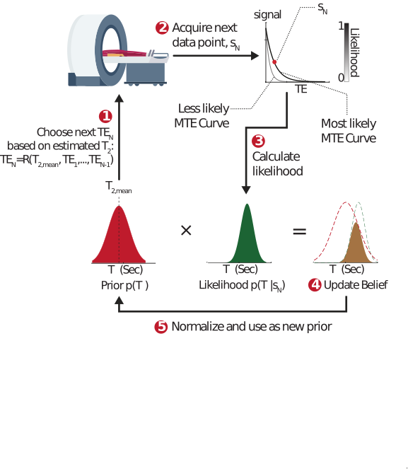
Pulse sequence parameters are conventionally static: They are set in advance, in anticipation of a particular type of contrast and a range of biological tissue parameters (e.g. $$$T_1$$$ or $$$T_2$$$). We propose an alternative adaptive approach to magnetic resonance, where incoming patient data is used in real time to update the excitation parameters and personalize the tissue contrast to the subject inside the MRI scanner. This approach maintains a probability distribution, $$$p(T_2,...)$$$, which is updated after each excitation using a Bayesian probabilistic approach (Fig. 1). The updated distribution is used in turn to inform and sculpt the next excitation, creating a continuous, real-time interplay between the sequence and tissue parameters. We hypothesized this approach would lead to superior precision per unit time, and would allow for significant acceleration by acquiring fewer – but more informative – excitations.Theory
Adaptive approach: Our adaptive framework was applied to a relaxometry single-voxel MRS experiment which quantified the $$$T_2$$$ relaxation time of n-acetyl-aspartate (NAA), a small neuronal metabolite. In this acquisition, a single echo is acquired per excitation at a given echo time (TE). The signal behaves as $$$s(TE)=PD\cdot\exp(-TE/T_2)$$$, where PD is the proton density. The adaptive approach maintains a probability distribution $$$p(T_2, PD)$$$ which quantifies the assumed a‑priori probability of each value of the tissue parameters. Given such a distribution, we can estimate $$$T_2$$$ via $$$T_{2,est}=\int T_2p(T_2,PD)dT_2dPD$$$, which can be used - alongside all previously selected TEs - to minimize the Cramer Rao Lower Bound (CRLB) for the estimated $$$T_2$$$. A new data point $$$s_N=s(TE_N)$$$ is then acquired, and used to calculate the likelihood of each possible $$$T_2$$$ and PD value given the new measurement: $$$L(T_2, PD|s_N)=exp\left(-\left(\frac{s_N -s(TE_N)}{\sqrt{2}\sigma}\right)^2\right)$$$, assuming the data contains Gaussian white noise with zero mean and variance $$$σ^2$$$. The prior $$$p(T_2, PD)$$$ is then updated via Bayes’ rule: $$$p_{new}(T_2,PD)=p_{old}(T_2,PD){\cdot}L(T_2,PD|s_N)$$$, and normalized to unity. This calculation is carried out in real time each TR.Static Approach: Any adaptive approach must be compared to a static one, of equal total acquisition time. The static sequence parameters must be fixed in advance, in anticipation of a wide possible range of $$$T_2$$$ values. A static experiment optimizes the mean CRLB over this range.
Methods
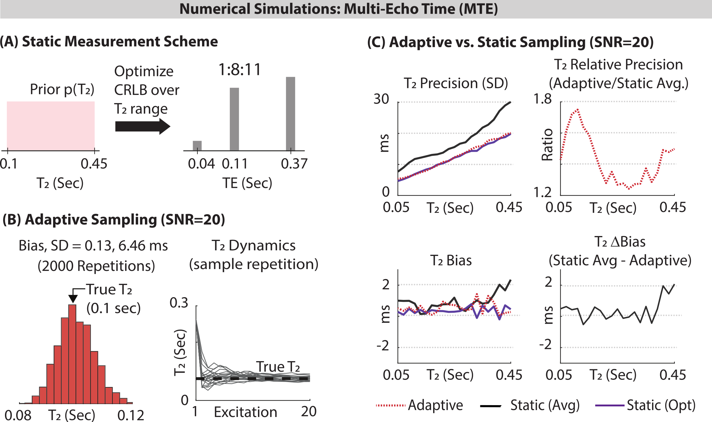
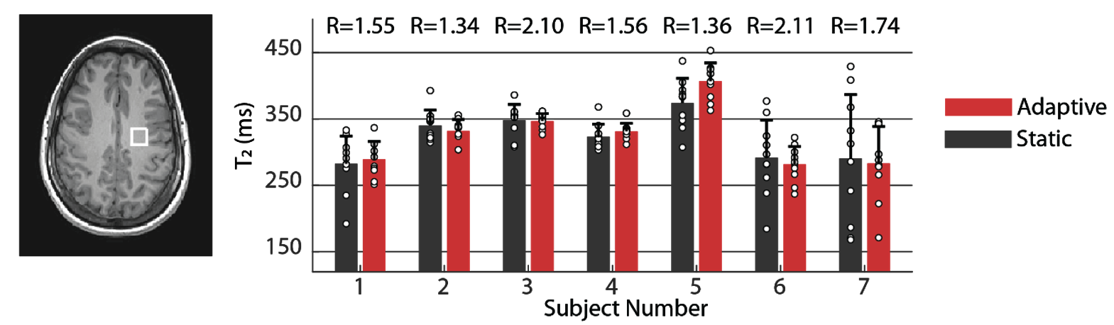
Simulations: Monte‑Carlo simulations were used to compare the bias and standard deviation of static and adaptive approaches (TA=2 min, TR=6 sec, 20 TEs). Static TEs which resulted from optimizing the mean CRLB were placed at 40, 110 and 370 ms at a 1:8:11 ratio (Fig. 2A). $$$T_2$$$ was fixed, and 2000 experiments were run for each approach, with different normally distributed generated noise (SNR=20). Each experiment yielded a single estimate for $$$T_2$$$. The 2000 $$$T_2$$$s were used to calculate the standard deviation and bias. This was repeated for different fixed values of $$$T_2$$$ between 0.05 and 0.45 seconds.In-Vivo: Seven healthy volunteers provided informed consent, approved by Wolfson Medical Center Helsinki committee. A $$$1.5\times1.5\times1.5 \textrm{cm}^3$$$ voxel was placed in parietal white matter. Twelve adaptive and twelve static acquisitions were interleaved, each lasting two minutes (12*2=24 minutes per approach). The adaptive scans targeted the $$$T_2$$$ relaxation time of the NAA singlet at 2.01 ppm. Each acquisition yielded a single $$$T_2$$$ estimate for NAA, resulting in twelve $$$T_2$$$ estimates per approach and volunteer. A linear mixed model tested for statistically significant differences between the two approaches, as well as estimate the intra-subject standard deviation for each approach. To determine the commensurate acceleration offered by the adaptive approach, we recalculated the mean precision of the adaptive MR dataset by taking successively fewer excitations (omitting later excitations), until further removal of excitations resulted in worse precision by the adaptive approach compared to the static approach.
Results
Simulations: Fig. 2C shows the absolute and relative bias of $$$T_2$$$ estimation for the adaptive and static approaches, as well as for an optimal approach in which the echo times were selected to minimize each $$$T_2$$$'s CRLB. Both approaches are unbiased, but the adaptive approach offers gains in precision from 1.2-1.8 (depending on $$$T_2$$$), and nearly matches the optimal approach.In-Vivo: Fig. 3 compares the estimated static and adaptive $$$T_2$$$ values for each volunteer. Methods' means were not statistically different, indicating both approaches yield the "same" estimate as expected. The mixed model revealed the standard deviation of the adaptive approach was 1.69-fold smaller than the static approach (p=0.0028). Retaining only 40% of the initial adaptive excitations resulted in equal standard deviations, demonstrating a potential 2.5-fold acceleration for the adaptive framework.
Discussion and Conclusion
Adaptive sequences, here demonstrated for $$$T_2$$$ relaxometry of NAA, offer a completely new venue for accelerating MR acquisitions several‑fold (herein 2.5-fold in-vivo). The proposed framework can be adopted to target any tissue property ($$$T_1$$$, $$$T_2$$$, diffusion, etc), and the gains obtained are completely independent of any other sources of acceleration (including compressed sensing, MR fingerprinting and parallel imaging).Recently, several suggestions have been made for adapting the k-space sampling patterns to match specific features of the objects being imaged. This general problem of designing optimal pairs of samplers and reconstruction strategies has led to several adaptive k‑space sampling paradigms based on machine learning, sometimes termed active MRI or sequential MRI [3-8]. This work complements them by targeting the excitation parameters.
Acknowledgements
The work was funded by the Israeli Science Foundation personal grant 416/20.References
[1] Moffett JR, Ross B, Arun P, Madhavarao CN, Namboodiri AM. N-Acetylaspartate in the CNS: from neurodiagnostics to neurobiology. Prog Neurobiol 2007;81(2):89-131.
[2] Kirov, II, Tal A. Potential clinical impact of multiparametric quantitative MR spectroscopy in neurological disorders: A review and analysis. Magn Reson Med 2020;83(1):22-44.
[3] Mardani M, Giannakis GB, Ugurbil K. Tracking Tensor Subspaces with Informative Random Sampling for Real-Time MR Imaging. arXiv e-prints 2016:arXiv:1609.04104. .
[4] He Z, Zhao B, Zhang Z. Active Sampling for Accelerated MRI with Low-Rank Tensors. arXiv e-prints 2020:arXiv:2012.12496. .
[4] Jin KH, Unser M, Moo Yi K. Self-Supervised Deep Active Accelerated MRI. arXiv e-prints 2019:arXiv:1901.04547.
[5] Zhang Z, Romero A, Muckley MJ, Vincent P, Yang L, Drozdzal M. Reducing Uncertainty in Undersampled MRI Reconstruction With Active Acquisition. 2019 15-20 June 2019. p 2049-2053.
[6] Bakker T, van Hoof H, Welling M. Experimental design for MRI by greedy policy search. In: Larochelle H, Ranzato M, Hadsell R, Balcan MF, Lin H, editors. Advances in Neural Information Processing Systems. Volume 33: Curran Associates, Inc.; 2020. p 18954-18966.
[7] Pineda L, Basu S, Romero A, Calandra R, Drozdzal M. Active MR k-space Sampling with Reinforcement Learning. In: Martel AL, Abolmaesumi P, Stoyanov D, Mateus D, Zuluaga MA, Zhou SK, Racoceanu D, Joskowicz L, editors; Cham. Springer International Publishing. p 23-33.
[8] Yin T, Wu Z, Sun H, Dalca AV, Yue Y, Bouman KL. End-to-End Sequential Sampling and Reconstruction for MRI. arXiv e-prints 2021:arXiv:2105.06460.
Figures