0069
What if every voxel was measured with a different diffusion protocol?1Center for Advanced Imaging Innovation and Research (CAI2R), Department of Radiology, New York University School of Medicine, New York, NY, United States, 2GE Research, Niskayuna, NY, United States
Synopsis
Keywords: Data Processing, Diffusion/other diffusion imaging techniques
A naive answer to this question is to loop over all voxels re-do the training and apply machine learning estimators of your favorite model. This is grossly computationally inefficient. We propose a matrix pseudoinversion-based method that can estimate nonlinear biophysical model parameters from a large set of voxels with independent acquisition protocols in a few minutes. Our framework can be tailored to any convolution-based model. Furthermore, the protocols are not required to have shells and there are no limits to the protocol differences among voxels. This method is readily extendable for simultaneously varying diffusion times, B-tensor shapes, TE, etc.Introduction
Recent advances in MRI gradient hardware, especially ultra-high efficient gradient coils1,2, have enabled high-gradient diffusion MRI (dMRI) in the human brain. Improving resolution3, sensitivity to axon diameters4, or achieving previously unexplored measurement regimes5 are only a subset of the exciting new opportunities that have become available. However, the price to pay for using such high-performance systems are gradient nonlinearities6, which may cause biases if unaddressed. Away from the isocenter, the applied diffusion weighting deviates from the nominal settings; this deviation further depends on the gradient direction. This means that actual protocols vary significantly from voxel to voxel, and may not even consist of shells in $$$q$$$-space.For biophysical models of white matter (WM)7-12 and gray matter13-15, the optimal parameter estimation at typical signal-to-noise ratios (SNR) has been shown to be a data-driven regression16,17. However, training a machine-learning parameter estimator for each voxel separately would involve up to a million of distinct protocols and is grossly computationally inefficient. Here we propose a matrix pseudoinversion-based method that is able to estimate nonlinear biophysical model parameters from a large set of voxels (e.g. whole brain) with independent acquisition protocols in a few minutes, with no constraints imposed on the acquisition design. The method relies on SVD-based separation between protocol parameters and model parameters in any model expression, such that the training is done only once on the model-parameter part, while the protocol-dependent part varying among voxels is handled with a linear regression.
Methods
Without loss of generality, consider the Standard Model (SM) of diffusion in WM. At long diffusion times WM can be modeled as a convolution over the sphere7-12:$$S\left(b,\hat{\mathbf{g}}\mid\,\!x,p_{\ell\!\,m}\right)=\int_{\mathbb{S}^{2}}d\hat{\mathbf{n}}\,\mathcal{K}(b,\hat{\mathbf{g}}\cdot\hat{\mathbf{n}}\mid\,\!x)\,\mathcal{P}(\hat{\mathbf{n}}\mid\,\!p_{\ell\,\!m}),\quad(1)$$
where $$$b$$$ and $$$\hat{\mathbf{g}}$$$ define the measurement, $$$x=[f,D_a,D_e^{||},D_e^{\perp},...]$$$ contains the parameters describing the fiber response $$$\mathcal{K}$$$ (kernel), and $$$\mathcal{P}(\hat{\mathbf{n}}\mid\,\!p_{\ell\,\!m})=\sum_{\ell\,\!m}p_{\ell\,\!m}\,Y_{\ell\,\!m}(\hat{\mathbf{n}})$$$ is the fiber orientation distribution function (fODF) with spherical harmonics coefficients $$$p_{\ell\,\!m}$$$. In spherical harmonics basis:
$$S\left(b,\hat{\mathbf{g}}\mid\,\!x,p_{\ell\!\,m}\right)=\sum_{\ell\,\!m}S_{\ell\,\!m}(b)\,Y_{\ell\,\!m}(\hat{\mathbf{g}})=\sum_{\ell\,\!m}\mathcal{K}_{\ell}(b\mid\,\!x)\,p_{\ell\,\!m}\,Y_{\ell\,\!m}(\hat{\mathbf{g}}).\quad(2)$$
where $$$\mathcal{K}_{\ell}$$$ are the kernel rotational invariants.
The key idea is to decouple tissue and protocol parameters, up to any desired accuracy, into orthogonal functions using singular value decomposition (SVD):
$$\mathcal{K}_\ell(b\mid\,\!x)\simeq\sum_{n=1}^{N_{\ell}}s_{n}^{(\ell)}\,u_{n}^{(\ell)}(b)\,v_{n}^{(\ell)}(x).\quad(3)$$
Substituting Eq. (3) into Eq. (2), we can write:
$$S\left(b,\hat{\mathbf{g}}\mid\,\!x,p_{\ell\!\,m}\right)\simeq\sum_{n\ell\,\!m}\underbrace{s_{n}^{(\ell)}\,u_{n}^{(\ell)}(b)\,Y_{\ell\,\!m}\left(\hat{\mathbf{g}}\right)}_{\alpha_{n\ell\,\!m}}\,\underbrace{v_{n}^{(\ell)}(x)\,p_{\ell\,\!m}}_{\gamma_{n\ell\,\!m}}=\sum_{n\ell\,\!m}\alpha_{n\ell\,\!m}(b,\hat{\mathbf{g}})\,\gamma_{n\ell\,\!m}(x,p_{\ell\,\!m}).\quad(4)$$
The spherical convolution and subsequent SVD factorization, allow us to write the diffusion signal as a product of data-driven basis functions $$$\alpha$$$ and $$$\gamma$$$. Here, $$$\alpha_{n\ell\,\!m}(b,\hat{\mathbf{g}})$$$ depends purely on the protocol parameters, while $$$\gamma_{n\ell\,\!m}(x,p_{\ell\,\!m})$$$ depends only on tissue (model) parameters.
This decoupling enables estimating
$$\hat{\gamma}_{n\ell\,\!m}=\alpha_{n\ell\,\!m}^\dagger(b,\hat{\mathbf{g}})\,S,\quad(5)$$
using linear Moore-Penrose pseudoinverse $$$\alpha_{\ell\,\!m n}^\dagger$$$ applied to a measurement $$$S$$$ in a given voxel. The estimated $$$\hat\gamma_{n\ell\,\!m}$$$ can subsequently be mapped to the corresponding set of kernel parameters. For that, we can use any data-driven regression to compute the mapping $$$\hat{\gamma}_{n\ell\,\!m}\rightarrow\,\!\{x,p_{\ell\,\!m}\}$$$ only once, as it is protocol-independent, and apply it to all brain voxels simultaneously in virtually no time.
The only computationally-intensive step is performing the protocol-dependent pseudoinverse $$$\alpha_{n\ell\,\!m}^\dagger(b,\hat{\mathbf{g}})$$$ for each voxel (which takes about the same time as, e.g. DTI or DKI estimation). For each voxel with a given protocol $$$(b,\hat{\mathbf{g}})$$$, we evaluate $$$\alpha_{n\ell\,\!m}(b,\hat{\mathbf{g}})$$$ based on Chebyshev interpolation18 of a pre-computed library of $$$u_{n}^{(\ell)}(b)$$$.
Experiments
This study was performed under a local IRB-approved protocol. After providing informed consent, a 44-year-old male volunteer underwent MRI in a 3T-system (GE Healthcare, WI, USA) using a MAGNUS head-only gradient insert1 and a 32-channel head coil. A monopolar PGSE diffusion weighting sequence was used for acquiring shells at $$$(b\,[\mathrm{ms/\mu\,\!m^2}],\,N_\mathrm{dirs})=\{(1,25);(2,60);(8,50)\}$$$, with $$$\Delta=23\,\mathrm{ms}$$$, $$$\delta=12\,\mathrm{ms}$$$. Imaging parameters: voxel size$$$\,=2\times2\times2\,$$$mm$$$^3$$$, $$$\mathrm{TE}=46\,\mathrm{ms}$$$, $$$\mathrm{TR}=5\,\mathrm{s}$$$, Echo-spacing$$$\,=\,424\,\mathrm{\mu\,\!s}$$$, in-plane acceleration$$$=2$$$, $$$\text{partial Fourier}\,=\,0.65$$$.Results
To recompute $$$\alpha_{n\ell\,\!m}(b,\hat{\mathbf{g}})$$$ values at each variation of the protocol, we generated a library of $$$u_{n}^{(\ell)}(b)$$$ consisting of 30000 random sets of SM parameters and 1000 b-values sampled at Chebyshev roots $$$\in[0,\, b_\mathrm{max}=15\mathrm{ms/\mu\,\!m^2}]$$$. This allowed accurate interpolation of $$$u_{n}^{(\ell)}(b)$$$ and subsequent approximation of $$$\mathcal{K}_\ell(b\mid\,\!x)$$$, see Fig. 1. To test the generalization of this library, we simulated SM signals from two arbitrary protocols (see Fig. 2), and performed the proposed estimation approachafter noise addition to $$$S$$$: $$$S(b,\hat{\mathbf{g}})\rightarrow\hat{\gamma}_{n\ell\,\!m}\rightarrow\,\!\{x,p_{\ell\,\!m}\}$$$.The in vivo data shows significant gradient nonlinearities. These can be observed by computing the re-scaling of the b-value as we traverse the FOV. This profile is specific to each diffusion direction, see Fig. 3a. We can recompute the corresponding protocol at each voxel and its $$$\alpha_{n\ell\,\!m}(b,\hat{\mathbf{g}})$$$. In Fig. 3b we show the spatial variation of the condition number of $$$\alpha_{n\ell\,\!m}(b,\hat{\mathbf{g}})$$$ after applying the voxelwise modifications to the nominal protocol. Figure 4 shows full brain maps of the linearly estimated $$$\hat{\gamma}_{n\ell\,\!m}$$$ parameters. Finally, Figure 5 shows SM parametric maps obtained from applying a fully connected neural network (100 neurons - 3 layers) to $$$\hat{\gamma}_{n\ell\,\!m}$$$.
Discussion and Conclusion
We proposed a machine learning parameter estimation framework that enables fast fitting of diffusion models to data where each voxel was acquired with a different protocol. This approach was trained only once, thus, significantly speeding up computation. We tested its feasibility on simulations and in vivo brain dMRI data acquired with a head-only gradient insert with significant gradient nonlinearities. Our framework can be tailored to any model based on a convolution of a fiber response and fODF. Furthermore, the data is not required to be sampled in shells and there are no limits to the gradient nonlinearities. This method is readily extendable for simultaneously varying diffusion times, B-tensor shapes, TE, etc.Acknowledgements
This work has been supported by NIH under NINDS award R01 NS088040 and NIBIB awards R01 EB027075 and P41 EB017183. The authors are grateful to Sune N. Jespersen for fruitful discussions and Nastaren Abad, Eric Fiveland, Maggie Fung, and Chitresh Bhushan for their help on the MRI experiments.References
[1] T. K. F. Foo, E. T. Tan, M. E. Vermilyea, Y. Hua, E. W. Fiveland, J. E. Piel, K. Park, J. Ricci, P. S. Thompson, D. Graziani, G. Conte, A. Kagan, Y. Bai, C. Vasil, M. Tarasek, D. T. Yeo, F. Snell, D. Lee, A. Dean, J. K. DeMarco, R. Y. Shih, M. N. Hood, H. Chae, and V. B. Ho, “Highly efficient head-only magnetic field insert gradient coil for achieving simultaneous high gradient amplitude and slew rate at 3.0t (MAGNUS) for brain microstructure imaging,” Magnetic Resonance in Medicine, vol. 83, no. 6, pp. 2356–2369, 2020.
[2] S. Y. Huang, T. Witzel, B. Keil, A. Scholz, M. Davids, P. Dietz, E. Rummert, R. Ramb, J. E. Kirsch, A. Yendiki,Q. Fan, Q. Tian, G. Ramos-Llord ́en, H.-H. Lee, A. Nummenmaa, B. Bilgic, K. Setsompop, F. Wang, A. V. Avram,M. Komlosh, D. Benjamini, K. N. Magdoom, S. Pathak, W. Schneider, D. S. Novikov, E. Fieremans, S. Tounekti, C. Mekkaoui, J. Augustinack, D. Berger, A. Shapson-Coe, J. Lichtman, P. J. Basser, L. L. Wald, and B. R. Rosen, “Connectome 2.0: Developing the next-generation ultra-high gradient strength human MRI scanner for bridging studies of the micro-, meso- and macro-connectome,” NeuroImage, vol. 243, p. 118530, 2021.
[3] J. A. McNab, B. L. Edlow, T. Witzel, S. Y. Huang, H. Bhat, K. Heberlein, T. Feiweier, K. Liu, B. Keil, J. Cohen-Adad, M. D. Tisdall, R. D. Folkerth, H. C. Kinney, and L. L. Wald, “The human connectome project and beyond: Initial applications of 300mt/m gradients,” NeuroImage, vol. 80, pp. 234–245, 2013.
[4] J. Veraart, D. Nunes, U. Rudrapatna, E. Fieremans, D. K. Jones, D. S. Novikov, and N. Shemesh, “Noninvasivequantification of axon radii using diffusion MRI,” eLife, vol. 9, p. e49855, 2020.
[5] H.-H. Lee, D. S. Novikov, and E. Fieremans, “Localization regime of diffusion in human gray matter on a high-gradient MR system: Sensitivity to soma size,” vol. 0639, 2022.
[6] D. Jones, D. Alexander, R. Bowtell, M. Cercignani, F. Dell’Acqua, D. McHugh, K. Miller, M. Palombo, G. Parker,U. Rudrapatna, and C. Tax, “Microstructural imaging of the human brain with a ‘super-scanner’: 10 key advantages of ultra-strong gradients for diffusion MRI,” NeuroImage, vol. 182, pp. 8–38, 2018. Microstructural Imaging.
[7] D. S. Novikov, E. Fieremans, S. N. Jespersen, and V. G. Kiselev, “Quantifying brain microstructure with diffusion MRI: Theory and parameter estimation,” NMR in Biomedicine, p. e3998, 2019.
[8] C. D. Kroenke, J. J. Ackerman, and D. A. Yablonskiy, “On the nature of the naa diffusion attenuated MR signal in the central nervous system,” Magnetic Resonance in Medicine, vol. 52, no. 5, pp. 1052–1059, 2004.
[9] S. N. Jespersen, C. D. Kroenke, L. Østergaard, J. J. H. Ackerman, and D. A. Yablonskiy, “Modeling dendrite density from magnetic resonance diffusion measurements,” NeuroImage, vol. 34, pp. 1473–1486, 2007.
[10] E. Fieremans, J. H. Jensen, J. A. H. ans Sungheon Kim, R. I. Grossman, M. Inglese, and D. S. Novikov, “Diffusiondistinguishes between axonal loss and demyelination in brain white matter,” in Proceedings of the International Society of Magnetic Resonance in Medicine, Wiley, 2012.
[11] H. Zhang, T. Schneider, C. A. Wheeler-Kingshott, and D. C. Alexander, “NODDI: Practical in vivo neurite orientation dispersion and density imaging of the human brain,” NeuroImage, vol. 61, pp. 1000–1016, 2012.
[12] J. H. Jensen, G. Russell Glenn, and J. A. Helpern, “Fiber ball imaging,” NeuroImage, vol. 124, pp. 824–833, 2016.
[13] M. Palombo, A. Ianus, M. Guerreri, D. Nunes, D. C. Alexander, N. Shemesh, and H. Zhang, “SANDI: A compartment-based model for non-invasive apparent soma and neurite imaging by diffusion MRI,” NeuroImage, vol. 215, p. 116835, 2020.
[14] I. O. Jelescu, A. de Skowronski, F. Geffroy, M. Palombo, and D. S. Novikov, “Neurite exchange imaging (NEXI): A minimal model of diffusion in gray matter with inter-compartment water exchange,” NeuroImage, vol. 256,p. 119277, 2022.
[15] J. L. Olesen, L. Østergaard, N. Shemesh, and S. N. Jespersen, “Diffusion time dependence, power-law scaling, and exchange in gray matter,” NeuroImage, vol. 251, p. 118976, 2022.
[16] M. Reisert, E. Kellner, B. Dhital, J. Hennig, and V. G. Kiselev, “Disentangling micro from mesostructure by diffusion MRI: A Bayesian approach,” NeuroImage, vol. 147, pp. 964 – 975, 2017.
[17] S. Coelho, E. Fieremans, and D. S. Novikov, “How do we know we measure tissue parameters, not the prior?,” in Proceedings of the International Society of Magnetic Resonance in Medicine, Wiley, 2021.
[18] L. N. Trefethen, Approximation Theory and Approximation Practice, Extended Edition. Society for Industrial and Applied Mathematics, 2019.
Figures
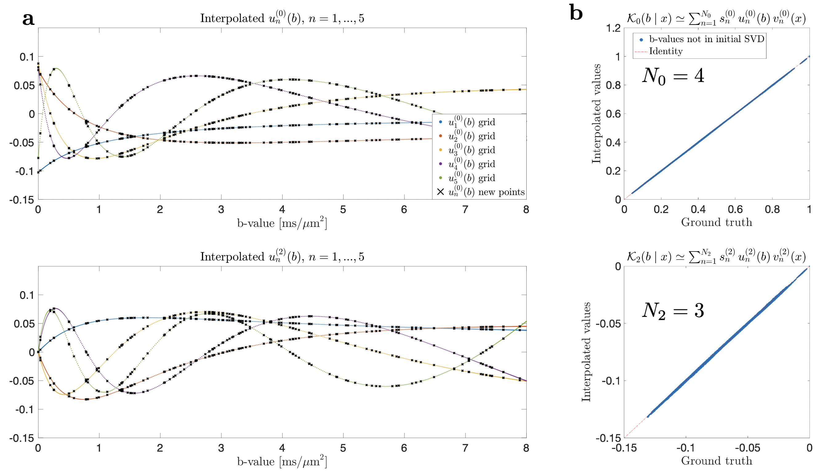
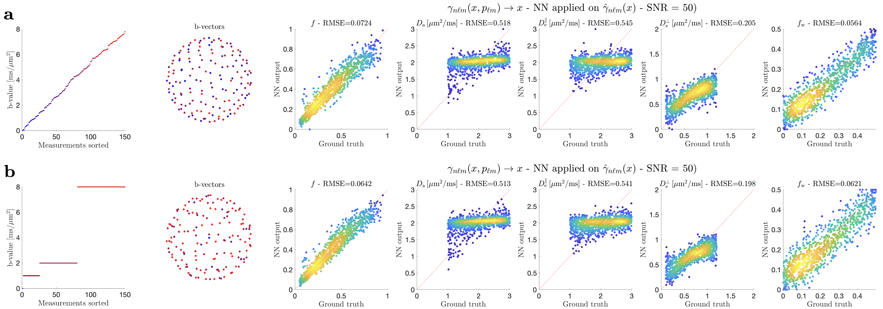
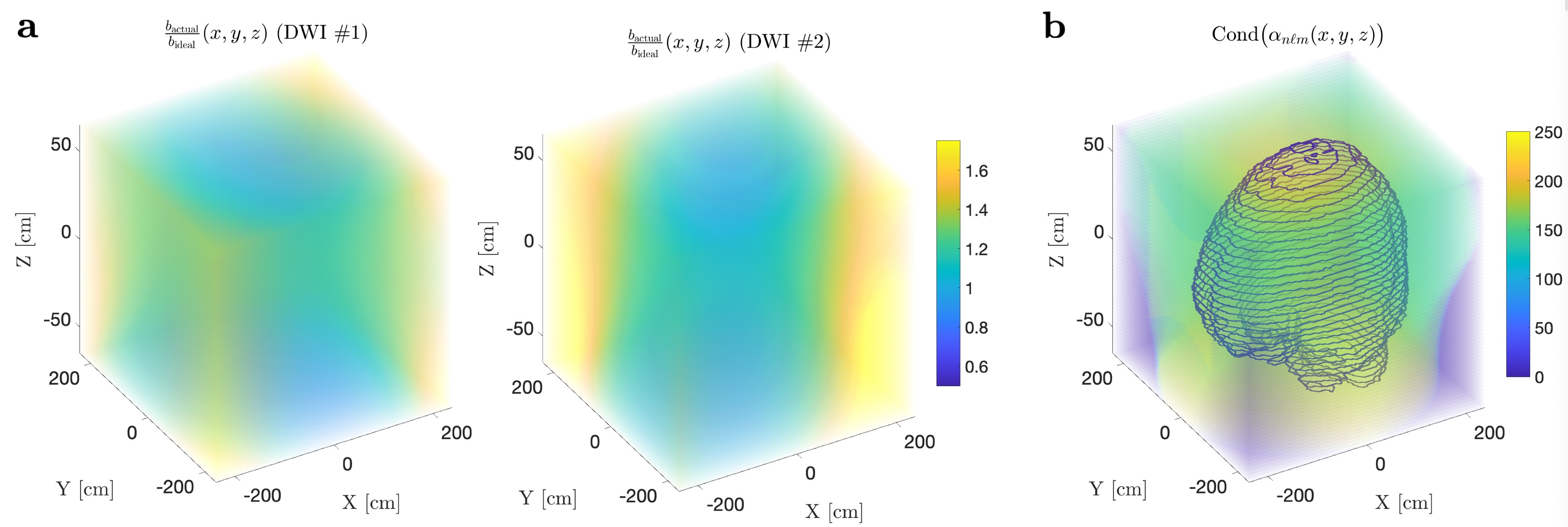
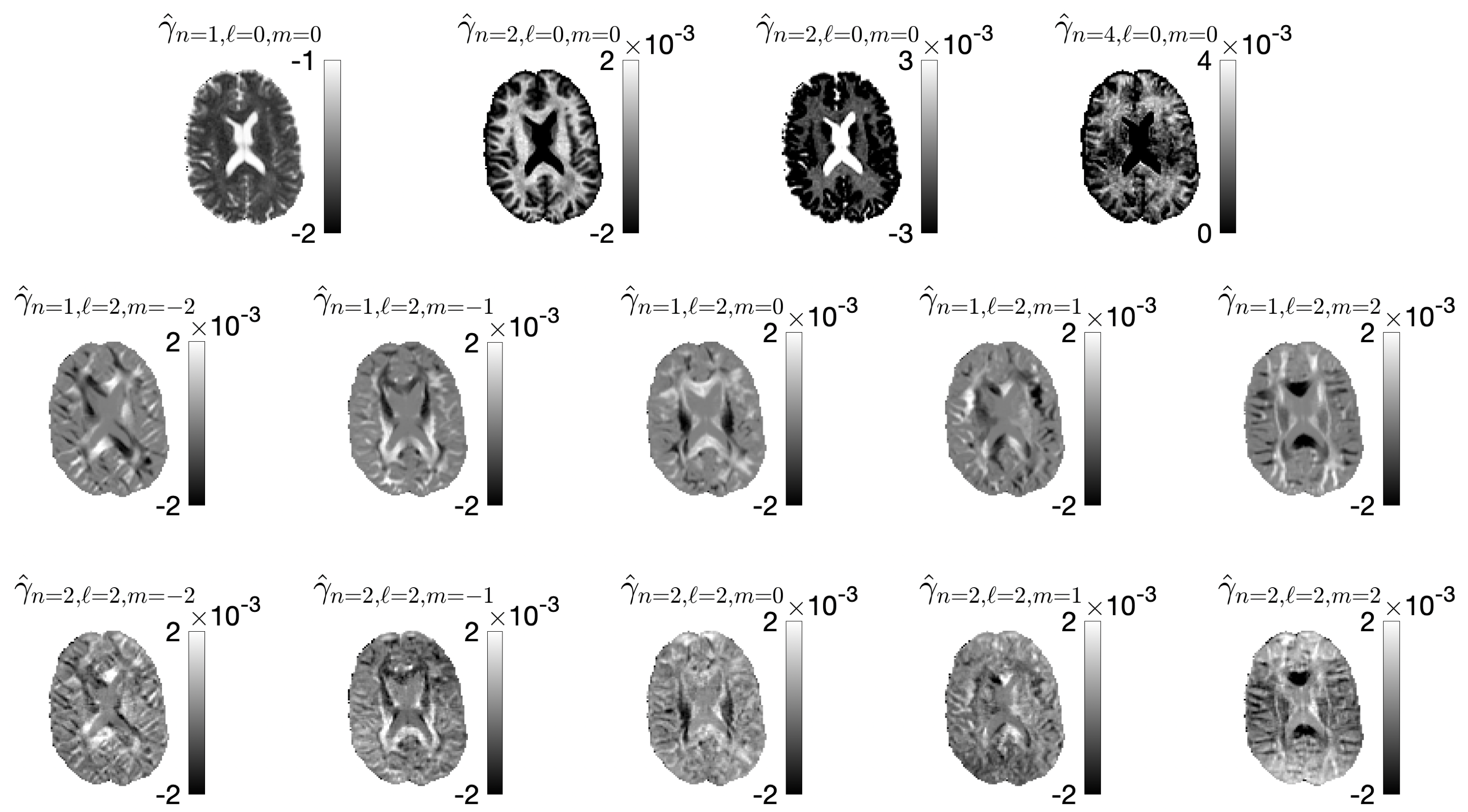
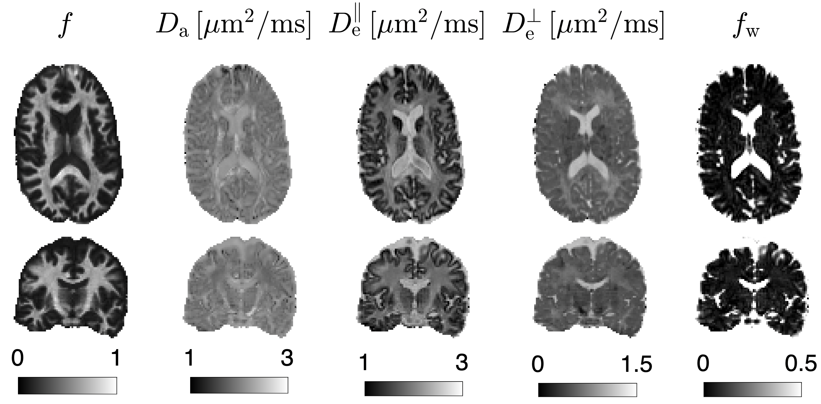
Figure 5. SMI maps are shown for transversal and coronal slices. These maps were obtained by applying a fully connected neural network on the $$$\hat{\gamma}_{n\ell\,\!m}$$$ shown in Fig. 4. Note that these biophysical parameters are only valid for the WM.