Overview

The Bloch equations describe the evolution of nuclear magnetization in response to applied magnetic fields. MR pulse sequences typically consist of multiple pulses of both RF and gradient fields, and recovery periods; simulation of the magnetization dynamics throughout a sequence involves integration of the Bloch equations through time during such a sequence.These simulations are an essential tool for evaluating expected contrast (hence designing sequences) and quantitative approaches which seek to relate the observed magnetization response to underlying tissue properties. Extended phase graphs (EPGs) are a powerful formalism for developing a qualitative understanding of signal formation, and for making numerical predictions. This talk will introduce the concepts behind EPGs and give some examples for their qualitative and quantitative use.

Echoes as an ensemble property

A general pulse sequence consists of RF pulses interspersed with applied field gradients, which are often not balanced (i.e. the gradients have nonzero zeroth moment). In this case we cannot simulate the signals that we would expect to receive by considering only the response of a single magnetization vector. Instead we must keep track of the behaviour of whole ensembles in order to recreate the ‘echoes’ that are key to the observed contrast. There are broadly speaking two ways to simulate such behaviour. The first is to sub-divide space into an ensemble of ‘isochromats’ which can be defined as regions in space where we can safely assume that the spins all experience the same Larmor frequency (the name derives from Greek and literally means ‘the same colour’). We can safely assume that each isochromat’s dynamics can be modelled using the Bloch equations, and then compute the net signal by summing up the transverse magnetization from each one. As an example of this Figure 1 shows an ensemble of magnetization isochromats in a constant gradient field, exposed to 3 90° RF pulses. As the figure shows, we see some peaks in the observed signal (“echoes”) two of which are identified as a ‘spin echo’ and a ‘stimulated echo’. If you look closely at figure 1 you can see that these echoes occur because a subset of the isochromats are aligned in the transverse plane. However the distribution of these isochromat magnetization vectors can be confusing and doesn’t give us a clear insight into the formation of these different echoes.

Isochromat Ensembles

Let’s focus on the example of an imaging sequence with unbalanced gradient G. Each application of an unbalanced gradient causes a spreading of the transverse magnetization (‘dephasing’): the phase angle in the rotating frame $$$\psi$$$ can be related to the location of the isochromat $$$\mathbf{r}$$$ by $$$ \psi=-\gamma\int_0^\tau \mathbf{G}(t).\mathbf{r} dt$$$ We will have a range of $$$\psi$$$ across a voxel, and successive applications of RF pulses and unbalanced gradients leads to a complex sub-voxel magnetization distribution.

Extended Phase Graphs

The sub-voxel magnetization distribution can be simulated by ‘sampling’ it in space by simulating isochromat ensembles, but another approach is to instead characterise the ensemble by its Fourier spectrum over ‘configuration states’. The magnetization distribution $$$M_{xy}(\mathbf{r})$$$ and $$$M_{z}(\mathbf{r})$$$ can be written in terms of configuration states:
$$ F_+(\mathbf{k}) = \int_V M_{xy}e^{-i\mathbf{k.r}}d^3\mathbf{r}$$
$$ Z(\mathbf{k}) = \int_V M_{z}e^{-i\mathbf{k.r}}d^3\mathbf{r}$$
Where `V' represents the voxel. The observed signal is the integrated transverse magnetization over the voxel, i.e. it is $$$F_+(0)$$$. Sequences that have a repeating gradient structure will produce rather compact magnetization distributions in this domain. This can be seen by the form of the rotation around the z axis by angle $$$\psi$$$ due to the applied gradient, which could be rewritten as:
$$ \psi=-\gamma\int_0^\tau \mathbf{G}(t).\mathbf{r} dt = \mathbf{\Delta k . r}$$
The effect of this gradient on the configuration states is to shift the transverse states such that $$$F_+(\mathbf{k})\rightarrow F_+(\mathbf{k}+\mathbf{\Delta k})$$$; this is mathematically equivalent to rotating the transverse magnetization around the z-axis, which is what happens in the space domain. If the same gradient area is applied after each excitation then the only possible values of k that can occur are integer multiples of Δk. In that case the magnetization can instead be written as the sum over a discrete set of configuration states:
$$M_{xy}(\psi)=\sum_{n=−∞}^∞ F_n e^{in\psi}$$
To fully understand the way that magnetization in the configuration states evolves through a sequence we also must consider the effect of RF pulses. In the isochromat domain an RF pulse causes the rotation of all magnetization vectors about some axis in the transverse plane, depending on the phase of the RF pulse. Crucially we consider the $$$B_1^+$$$ field to be uniform over the voxel, meaning that all isochromats in the ensemble are rotated by the same amount in the same direction. Hence an RF pulse cannot fundamentally alter the distribution of the magnetization, only rotate it. In the Fourier domain this means that an RF pulse will not `mix' configurations with different Δk; rather, RF pulses lead to a redistribution between longitudinal ($$$Z$$$) and transverse ($$$F$$$) configuration states with the same Δk. A fuller mathematical treatment will be given in the lecture; refer to [6] for an excellent in-depth introduction. The configuration states can be visualised as representing magnetization with different spatial modulation across a voxel; $$$F_0$$$ and $$$Z_0$$$ represent spatially constant magnetization, for example. Assuming that Δk imparts a phase of $$$2\pi$$$ across the voxel, all transverse configurations with n≠0 average to zero and hence $$$F_0$$$ represents the observed signal. $$$F_1$$$ and $$$Z_1$$$ represent magnetization modulated by $$$2\pi$$$ over the voxel, $$$F_2$$$ and $$$Z_2$$$ have twice this modulation, and so on as illustrated by Figure 2.

The EPG algorithm can be used to make quantitative signal simulations by repeatedly applying some simple rules: 1. RF pulses mix together $$$F_n$$$ and $$$Z_n$$$ with the same n; 2. gradients shift $$$F_n\rightarrow F_{n+1}$$$; 3. Relaxation is applied separately to each configuration using the appropriate weighting (discussed in the talk). An example is given in Figure 3.

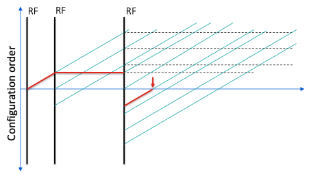
Returning to the 90°-90°-90° pulse sequence in Figure 1, we may evaluate this by drawing a phase graph diagram, Figure 4. The diagonal lines indicate the shifting of $$$F_+(k)$$$ to higher $$$k$$$ in the presence of a constant gradient. The red lines indicate the stimulated echo pathway, which represents spatially modulated magnetization that is rotated to the longitudinal direction, ‘storing’ this modulation in a $$$Z$$$ configuration. This is then rotated back into the transverse plane by the subsequent RF pulse and later measured as an echo. This type of diagram is a powerful way to understand and debug pulse sequences.

The EPG method is not inherently more computationally efficient than isochromat simulations for most operations. However an advantage is that the number of configurations that must be computed is well defined - we can see this by looking at the number of gradient periods. Perhaps more importantly, the EPG method allows us more \emph{insight} than isochromat simulations. We can see which `pathways' lead to echo formation, including more complex mechanisms such as stimulated echoes. Finally, we will briefly discuss how EPGs can be extended to model other effects, such as diffusion [5] or Magnetization Transfer and exchange [3].

Summary

Signal simulations are an essential part of MRI sequence development, and increasingly also required for quantitative MRI methods. Magnetization dynamics can be modelled by integrating the Bloch equations. Generally the action of gradients disperses magnetization within a voxel, and this complex sub-voxel distribution must be characterised in order to model the MRI signal. A general method is to divide space into infinitesimal portions that experience the same field (`isochromats'), model their magnetization separately, then integrate the result. The EPG method is an elegant alternative that performs the Bloch simulation in a Fourier domain representation that can be more compact, and can also give more insight into how signal properties arise in the first place.

Acknowledgements

No acknowledgement found.