Simulating Spectra
Jamie Near1
1Sunnybrook Research Institute, Canada
1Sunnybrook Research Institute, Canada
Synopsis
The goal of this lecture is to describe how to perform MR spectroscopy simulations using the density matrix formalism. The following questions will be addressed:
-What is a density matrix and how is it constructed?
-What is a Hamiltonian operator and how is it constructed?
-How does the density matrix evolve under the influence of Hamiltonian operators?
-How is a simple spin-echo simulation pulses performed?-How are shaped RF waveforms simulated?
-What are spatially-resolved simulations and how are they performed?
-What is the projection method and how does it work?
-What is coherence order filtering and how does it work?
Introduction
Density matrix simulations allow us to accurately predict the spectral shape for a given spin system under specific experimental conditions (field strength, pulse sequence, timing, etc). Though they may be intimidating at first, learning how to use density matrix simulations is well worth the effort. One of the most important applications of the density matrix simulations is for generating accurate basis sets for MRS quantification. But simulations are also very useful for quickly generating figures or illustrations, and for understanding and interpreting the results of MRS experiments.Methods
The density matrix, $$$σ$$$, is a matrix representation of the state of a spin system at a particular instant in time. In the same way that a sample magnetisation evolves under the influence of different pulse sequence elements, the density matrix evolves under the influence of so-called "Hamiltonian operators" which represent the various elements of the pulse sequence (RF pulses and delays). Density matrix evolution is carried out using the Louisville von Neumann Equation:$$σ(t)=exp(-iHt)σ(0) exp(iHt) [1]$$
in which the starting density matix, $$$σ(0)$$$, is sandwiched between two matrix exponentials with $$$-iHt$$$ and $$$+iHt$$$ as the arguments, respectively, where H is a so-called time-independent Hamiltonian operator.
For a system with N spins, the density matrix, is a $$$2^N * 2^N$$$ matrix, and can be described as a linear combination of 22N independent basis states. So, for a one-spin system, $$$σ$$$ is a 2 x 2 matrix and there are four basis matrices, as shown in Figure 1. These are called the Pauli Spin Matrices. $$$I_x$$$, $$$I_y$$$, and $$$I_z$$$ represent pure x, y and z magnetization, respectively, for a one-spin system1,2. Since at equilibrium the magnetization is orientated in the z-direction, the equilibrium density matrix is $$$I_z$$$.
For a 2-spin system ($$$I$$$ and $$$S$$$), the density matrix has dimensions 4 x 4 and there are 16 basis matrices. The basis matrices consist of all possible combinations of $$$I_0$$$, $$$I_x$$$, $$$I_y$$$, and $$$I_z$$$ with $$$S_0$$$, $$$S_x$$$, $$$S_y$$$, and $$$S_z$$$, i.e. $$$I_0 S_0$$$, $$$I_0 S_x$$$, $$$I_0 S_y$$$, $$$I_0 S_z$$$, $$$I_x S_0$$$, $$$I_x S_x$$$, $$$I_x S_y$$$, and so on. These two-spin basis matrices are sometimes called “product operators” and are obtained by taking the direct product (also known as the “Kroneker product”) of the corresponding one-spin Pauli spin matrices. For example, the matrix $$$I_z S_0$$$ is shown in Figure 2.
Hamiltonian operators describe pulse sequence events that can change the state of a spin system. The two main types of Hamiltonian operators that we need are: rotation operators (Hrot_x, Hrot_y), for simulating the effect of RF pulses; and free evolution operators (Hevol) for simulating the effects of delays or free evolution periods (i.e. rotations about the B0 field).
In this presentation, I will describe the Hamiltonian operators in more detail, and show how they are used to evolve the density matrix according to specifically designed pulse sequences. I will describe how a final FID signal is obtained from the evolved density matrix.
Some practicalities will also be covered in this talk, such as: How to account for shaped RF pulses, how to account for chemical shift displacement using spatially resolved simulations (see Figure 3), how to remove spectral contamination from unwanted coherences or outer volume signals, and how to accelerate simulations to reduce computation time.
Conclusion
Spectral simulation is a powerful technique that allows us to predict the spectral shape of any spin system under the influence of any pulse sequence. It is an indispensable tool for generating basis sets for quantification of in-vivo MRS data. It is also useful for generating figures and illustrations, and as a tool for understanding the MRS signal. The mathematics of density matrix simulations can be daunting at first, but with the help of a computational software such as MATLAB or similar, it is not too difficult to implement, and well worth the effort.Acknowledgements
Thank you to Robin Simpson, Chathura Kumaragamage, Richard Edden Georg Oeltzschner, Kimberly Chan, and Dana Goerzen and Brenden Kadota, who all helped me better understand density matrix simulations.References
1. Farrar, T.C. (1990). Density Matrices in NMR Spectroscopy: Part I. Concepts Magn Reson 2, 1-12.2. Farrar, T.C. (1990). Density Matrices in NMR Spectroscopy: Part II. Concepts Magn Reson 2, 55-61.
3. Zhang, Y., An, L., and Shen, J. (2017). Fast computation of full density matrix of multispin systems for spatially localized in vivo magnetic resonance spectroscopy. Med Phys 44, 4169-4178.
4. Landheer, K., Swanberg, K.M., and Juchem, C. (2021). Magnetic resonance Spectrum simulator (MARSS), a novel software package for fast and computationally efficient basis set simulation. NMR Biomed 34, e4129.
Figures
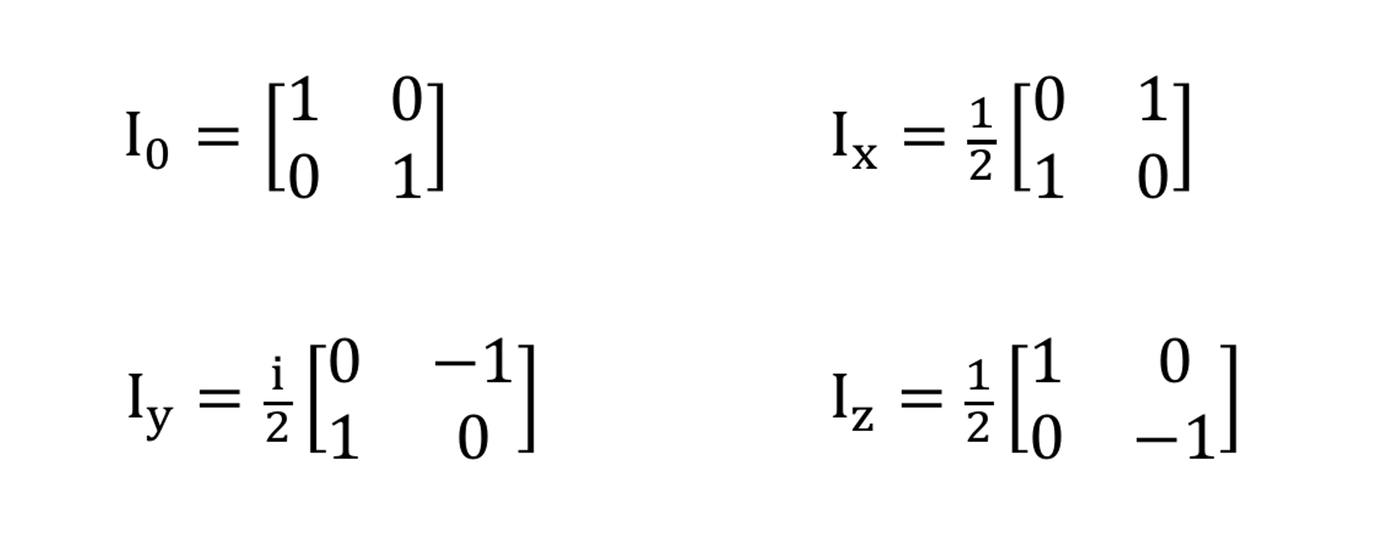
The Pauli Spin Matrices, forming the basis state matrices for a one-spin system.
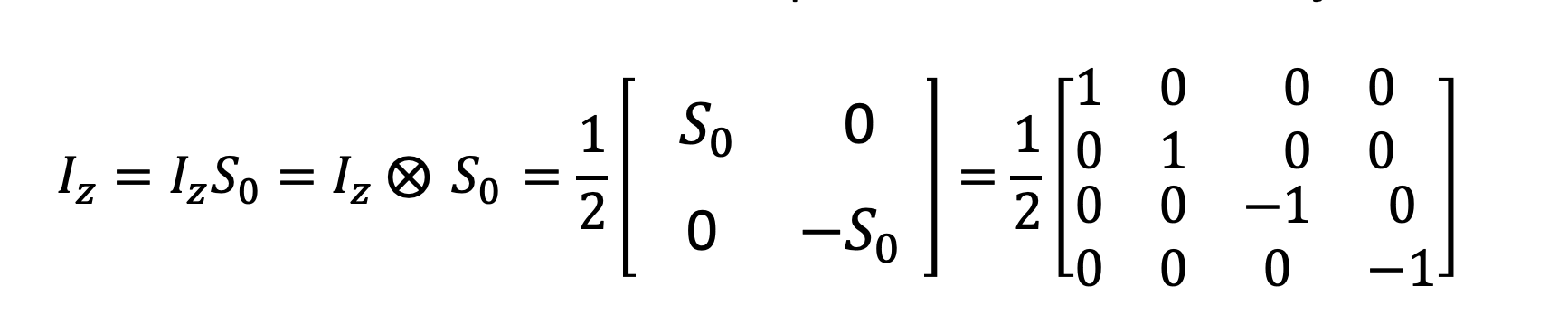
An example of a two-spin basis state: the I_z S_0 state (also known simply I_z). It is generated by taking the direct product (or Kroneker product) of the one-spin I_z matrix and the one-spin S_0 matrix.
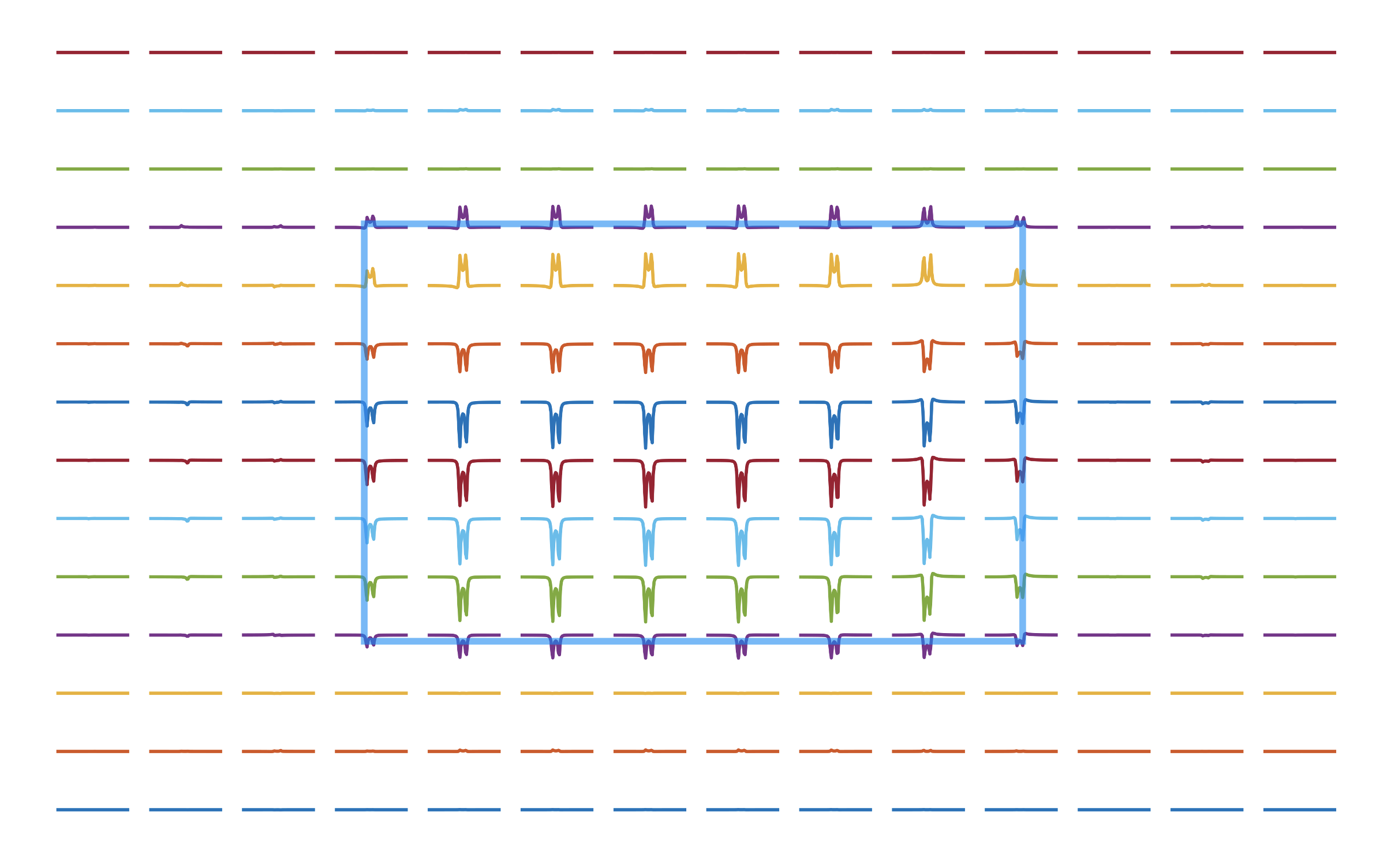
An example of a spatially-resolved PRESS simulation (TE=135ms) of Lactate following coherence order filtering. Only the 1.3 ppm resonance of Lactate is shown.