5050
Higher-order image reconstruction with integrated gradient nonlinearity correction using a low-rank encoding operator1Biomedical Engieering, University of Southern California, Los Angeles, CA, United States, 2Electrical Engieering, University of Southern California, Los Angeles, CA, United States
Synopsis
Conventional MR image reconstruction relies on the assumption of perfectly linear gradient fields. However, the gradient fields contain spatially varying nonlinear components. We present a higher-order image reconstruction method that incorporates a theoretical model of gradient nonlinearity without any external field monitoring device. This approach utilizes the separability of Fourier encoding in Cartesian imaging and employs a low-rank approximation only to the higher-order readout encoding matrix, allowing a memory-efficient implementation suitable for large FOVs. Image distortions due to gradient nonlinearity were successfully mitigated by the proposed method using axial/sagittal/coronal 2D Cartesian datasets acquired on a prototype 0.55T MRI system.
Introduction
Conventional MR image reconstruction relies on the assumption of perfectly linear gradient fields. However, due to engineering limitations, the gradient fields contain spatially varying nonlinear components. The importance of gradient nonlinearity correction increases when imaging large fields of view (FOV) and with the recent development of large-bore systems1, high-performance gradient inserts2,3, and MR-based radiotherapy systems4,5. In this work, we introduce a higher-order image reconstruction method6 for gradient nonlinearity (GNL) correction that incorporates a vendor-provided theoretical model of gradient nonlinearity without any field monitoring device7,8. This approach utilizes a low-rank approximation to the higher-order readout encoding matrix9,10 such that FFTs can be leveraged.Theory
From the vendor-provided information, a nonlinear gradient field along the z-axis generated by gradient coil calculated at the reference gradient strength is modeled by a spherical harmonics expansion (up to 13 order)11–13: $$B_{z,n}^i(r,\theta,\phi)=\sum_{\ell=0}^{\infty}\sum_{m=0}^{\ell}\left(\frac{r}{R_0}\right)^n [\alpha_{\ell m}^{i}\cos(m\phi)+\beta_{\ell m}^{i}\sin(m\phi)]P_{\ell,m}(\cos\theta),$$ where $$$R_0$$$ is the radius of a gradient coil and x,y,z are spatial coordinates in the physical coordinate system (PCS). A spatiotemporal nonlinear gradient field along the x-axis generated by a time-varying gradient $$$G_x(t)$$$ can be calculated as:$$B_{z,n}^x(\mathbf{r},t)=\left(B_{z,n}^x(r,\theta,\phi)\frac{1}{G_{x,\mathrm{ref}}}\right)G_{x}(t):=\Delta x(\mathbf{r})G_{x}(t).$$Similarly, we have$$$B_{z,n}^y(\mathbf{r},t)=\Delta y(\mathbf{r})G_{y}(t)$$$ and $$$B_{z,n}^z(\mathbf{r},t)=\Delta z(\mathbf{r})G_{z}(t)$$$. The magnitude of an applied magnetic field for the i-th phase encode can be represented as a sum of linear and nonlinear gradient fields:$$\begin{equation*}\begin{split}\|B_{z,n}^x(\mathbf{r},t)\|_{\ell_2}&=B_0+\mathbf{G}_i(t)\cdot\mathbf{r}+\Delta x(\mathbf{r})G_{x,i}(t)+\Delta y(\mathbf{r})G_{y,i}(t)+\Delta z(\mathbf{r})G_{z,i}(t)\\&=B_0+\mathbf{G}_{\mathrm{LCS},i}(t)\cdot\mathbf{r}_{\mathrm{LCS}}+\mathbf{G}_{\mathrm{LCS},i}(t)\cdot\mathbf{\Delta r}_{\mathrm{LCS}}(\mathbf{r}),\\\end{split}\end{equation*}$$ where in the last expression, gradients and spatial coordinates are transformed from the PCS to the logical coordinate system (LCS) (u=PE, v=RO, w=SL). The phase evolution for Cartesian imaging can be simplified because readout is the same for all phase encodes and the i-th phase encode is constant over the readout duration:$$\begin{equation*}\begin{split}\phi_i(\mathbf{r},t)&=\mathbf{k}_{\mathrm{LCS},i}(t)\cdot\mathbf{r}_{\mathrm{LCS}}+\mathbf{k}_{\mathrm{LCS},i}(t)\cdot\mathbf{\Delta r}_{\mathrm{LCS}}(\mathbf{r})\\&=k_u(t)u+k_v(t)v+k_{u,i}(t)\Delta u(\mathbf{r})+k_{v,i}(t)\Delta v(\mathbf{r}).\end{split}\end{equation*}$$Therefore, a signal encoding model for the i-th phase encode and c-th coil can be represented as$$\mathbf{d}_{i,c}=\mathbf{E}_i\mathbf{S}_c\mathbf{m}=\left(\mathbf{F}_u\odot\mathbf{F}_{v,i}\odot\mathbf{H}_u\odot\mathbf{H}_{v,i}\right)\mathbf{S}_c\mathbf{m},$$where $$$\odot$$$ represents the Hadamard product. Using a low-rank approximation to the higher-order readout encoding matrix, $$$\sum_{\ell=1}^L\mathbf{u}_{\ell}\mathbf{v}_{\ell}^H$$$, and exploiting the structure of $$$\mathbf{H}_{v,i}=\mathbf{1}_{N_k}\mathbf{h}_{v,i}^H$$$ and $$$\mathbf{F}_{v,i}=\mathbf{1}_{N_k}\mathbf{f}_{v,i}^H$$$, where $$$\mathbf{1}_{N_k}=[1,...,1]^T\in \mathbb{R}^{N_k}$$$, the encoding matrix can be simplified to$$\mathbf{E}_i=\mathbf{F}_u\odot\sum_{\ell=1}^L\mathbf{u}_\ell\left(\mathbf{f}_{v,i}\odot\mathbf{h}_{v,i}\odot\mathbf{v}_{\ell}\right)^H=\sum_{\ell=1}^L\mathrm{diag}(\mathbf{u}_{\ell})\mathbf{F}_u\mathrm{diag}(\left(\mathbf{f}_{v,i}\odot\mathbf{h}_{v,i}\odot\mathbf{v}_{\ell}\right)^\ast).$$Image reconstruction was performed by solving the following cost function:$$\hat{\mathbf{m}}=\underset{\mathbf{m}}{\mathrm{argmin}}\sum_{i=1}^{N_i}\sum_{c=1}^{N_c}\|\mathbf{d}_{i,c}-\mathbf{E}_i\mathbf{S}_c\mathbf{m}\|_{\ell_2}^2.$$Methods
Experimental Methods: Experiments were performed using a whole body 0.55T system (prototype MAGNETOM Aera, Siemens Healthineers, Erlangen, Germany) equipped with high-performance shielded gradients (45 mT/m amplitude, 200 T/m/s slew rate)14.Phantom experiments: Cartesian (axial, sagittal, coronal) scans of a NIST/ISMRM system phantom15 were acquired with a 2D GRE pulse sequence. Vendor-provided GNL correction via image-domain interpolation was applied16. Surface coil intensity correction was performed with the “Prescan Normalize” method17.
Axial imaging (x and y gradients): In-vivo human brain axial scans were acquired with a 2D multi-slice T2-weighted turbo spin echo (TSE) pulse sequence. Imaging parameters were refocusing FA=180°, TR=6500ms, TE=86ms, echo spacing=12.66ms, averages=2, resolution=0.72x0.72mm2, slice-thickness=5mm, and FOV=320x320mm2.
Sagittal imaging (y and z gradients): T1-weighted and in-vivo human spine sagittal scans were acquired with a 2D multi-slice FSE pulse sequence. Imaging parameters were refocusing FA=180°, TR=900ms, TE=13ms, TI=100ms, echo spacing=12.66ms, averages=2, resolution=0.75x0.75mm2, slice-thickness=4.5mm, and FOV=320x320mm2.
Coronal imaging (x and z gradients): In-vivo human lung coronal scans were acquired with a 2D single-slice balanced steady-state free precession (bSSFP) pulse sequence. Imaging parameters were FA=60°, TE=1.62ms, TR=3.24ms, resolution=3.28x3.28mm2, slice-thickness=15mm, and FOV=420x571mm2.
Results
Figure 1 shows higher-order image reconstruction with integrated GNL correction on three datasets (axial, coronal, sagittal) of a NIST/ISMRM system phantom. Note that even within a 10-cm distance from isocenter, gradient nonlinearity causes noticeable geometric distortions in the sagittal slice. Figure 2 shows higher-order image reconstruction with integrated GNL correction on the axial brain T2-weighted TSE scans. The DICOM images were processed with GNL correction, surface coil intensity correction, and advanced denoising18 and thus custom image reconstructions do not have identical image intensity and appearance. However, the proposed approach achieved high geometric fidelity comparable to the DICOM images. Figure 3 shows higher-order image reconstruction with integrated GNL correction on the sagittal spine T1-weighted TSE scans. A circular mask of radius 250 mm was applied to displacement fields as recommended by a vendor. The proposed approach successfully mitigated image distortions due to gradient nonlinearity at large FOV. Figure 4 shows higher-order image reconstruction with integrated GNL correction on the coronal lung bSSFP scans. The proposed approach resolved gradient nonlinearity with increased severity in off-center Cartesian imaging.Discussion
The proposed approach depends on the accuracy of the vendor-provided parameterization of the nonlinear gradient fields (e.g., highest harmonic order), whereas NMR field probes7,8 can provide greater accuracy with a larger number of spatially distinct field measurements. The reconstruction time of the proposed approach is slow compared with conventional parallel imaging techniques because many FFTs (L times) are required for each readout. The proposed approach could be beneficial to applications with large FOV such as body composition, fetal imaging, and abdominal imaging in obese subjects because image-domain GNL correction is known to cause blurring or resolution loss19. The ability to incorporate gradient nonlinearity into the theoretical derivation of concomitant fields20 may improve the applications that are affected by concomitant fields, including spiral imaging, water-fat separated imaging21,22, and T2* imaging23.Conclusion
Gradient nonlinearity can be incorporated into higher-order image reconstruction (e.g., expanded encoding model), and retains the ability to be accelerated using low-rank approximation. We demonstrate the power of this approach for brain, spine, and lung Cartesian imaging on a whole-body 0.55T system.Acknowledgements
We acknowledge grant support from the National Science Foundation (#1828736) and research support from Siemens Healthineers.References
1. Siemens Healthineers moves into new clinical fields with its smallest and most lightweight whole-body MRI. https://www.siemens-healthineers.com/press/releases/magnetom-free-max.html.
2. Lee SK, Mathieu JB, Graziani D, et al. Peripheral nerve stimulation characteristics of an asymmetric head-only gradient coil compatible with a high-channel-count receiver array. Magn. Reson. Med. 2016;76:1939–1950 doi: 10.1002/mrm.26044.
3. Weiger M, Overweg J, Rösler MB, et al. A high-performance gradient insert for rapid and short-T2 imaging at full duty cycle. Magn. Reson. Med. 2018;79:3256–3266 doi: 10.1002/mrm.26954.
4. Shan S, Liney GP, Tang F, et al. Geometric distortion characterization and correction for the 1.0 T Australian MRI-linac system using an inverse electromagnetic method. Med. Phys. 2020;47:1126–1138 doi: 10.1002/mp.13979.
5. Mutic S, Dempsey JF. The ViewRay System: Magnetic Resonance-Guided and Controlled Radiotherapy. Semin. Radiat. Oncol. 2014;24:196–199 doi: 10.1016/j.semradonc.2014.02.008.
6. Wilm BJ, Barmet C, Pavan M, Pruessmann KP. Higher order reconstruction for MRI in the presence of spatiotemporal field perturbations. Magn. Reson. Med. 2011;65:1690–1701 doi: 10.1002/mrm.22767.
7. De Zanche N, Barmet C, Nordmeyer-Massner JA, Pruessmann KP. NMR Probes for measuring magnetic fields and field dynamics in MR systems. Magn. Reson. Med. 2008;60:176–186 doi: 10.1002/mrm.21624.
8. Barmet C, De Zanche N, Pruessmann KP. Spatiotemporal magnetic field monitoring for MR. Magn. Reson. Med. 2008;60:187–97 doi: 10.1002/mrm.21603.
9. Wilm BJ, Barmet C, Pruessmann KP. Fast higher-order MR image reconstruction using singular-vector separation. IEEE Trans. Med. Imaging 2012 doi: 10.1109/TMI.2012.2190991.
10. Fessler JA, Lee S, Olafsson VT, Shi HR, Noll DC. Toeplitz-based iterative image reconstruction for MRI with correction for magnetic field inhomogeneity. IEEE Trans. Signal Process. 2005;53:3393–3402 doi: 10.1109/TSP.2005.853152.
11. Krieg R, Schreck O. Method for three-dimensionally correcting distortions and magnetic resonance apparatus for implementing the method. U.S. patent no. 6501273. 2002.
12. Janke A, Zhao H, Cowin GJ, Galloway GJ, Doddrell DM. Use of spherical harmonic deconvolution methods to compensate for nonlinear gradient effects on MRI images. Magn. Reson. Med. 2004;52:115–122 doi: 10.1002/mrm.20122.
13. Jovicich J, Czanner S, Greve D, et al. Reliability in multi-site structural MRI studies: Effects of gradient non-linearity correction on phantom and human data. Neuroimage 2006;30:436–443 doi: 10.1016/j.neuroimage.2005.09.046.
14. Campbell-Washburn AE, Ramasawmy R, Restivo MC, et al. Opportunities in interventional and diagnostic imaging by using high-performance low-field-strength MRI. Radiology 2019;293:384–393 doi: 10.1148/radiol.2019190452.
15. Stupic KF, Ainslie M, Boss MA, et al. A standard system phantom for magnetic resonance imaging. Magn. Reson. Med. 2021;86:1194–1211 doi: 10.1002/mrm.28779.
16. Krieg R. Method of distortion correction for gradient non-linearities in nuclear magnetic resonance tomography apparatus. U.S. patent no. 5886524. 1999.
17. Kremers FPPJ, Hofman MBM, Groothuis JGJ, et al. Improved correction of spatial inhomogeneities of surface coils in quantitative analysis of first-pass myocardial perfusion imaging. J. Magn. Reson. Imaging 2010;31:227–233 doi: 10.1002/jmri.21998.
18. Kannengiesser SAR, Mailhe B, Nadar M, Huber S, Kiefer B. Universal iterative denoising of complex-valued volumetric MR image data using supplementary information. Proc Intl Soc Mag Reson Med 2016:4–6.
19. Tao S, Trzasko JD, Shu Y, Huston J, Bernstein MA. Integrated image reconstruction and gradient nonlinearity correction. Magn. Reson. Med. 2015;74:1019–1031 doi: 10.1002/mrm.25487.
20. Testud F, Gallichan D, Layton KJ, et al. Single-shot imaging with higher-dimensional encoding using magnetic field monitoring and concomitant field correction. Magn. Reson. Med. 2015;73:1340–1357 doi: 10.1002/mrm.25235.
21. Colgan TJ, Hernando D, Sharma SD, Reeder SB. The effects of concomitant gradients on chemical shift encoded MRI. Magn. Reson. Med. 2017;78:730–738 doi: 10.1002/mrm.26461.
22. Ruschke S, Eggers H, Kooijman H, et al. Correction of phase errors in quantitative water–fat imaging using a monopolar time-interleaved multi-echo gradient echo sequence. Magn. Reson. Med. 2017;78:984–996 doi: 10.1002/mrm.26485.
23. Hofstetter LW, Morrell G, Kaggie J, Kim D, Carlston K, Lee VS. T2* Measurement bias due to concomitant gradient fields. Magn. Reson. Med. 2017;77:1562–1572 doi: 10.1002/mrm.26240.
Figures
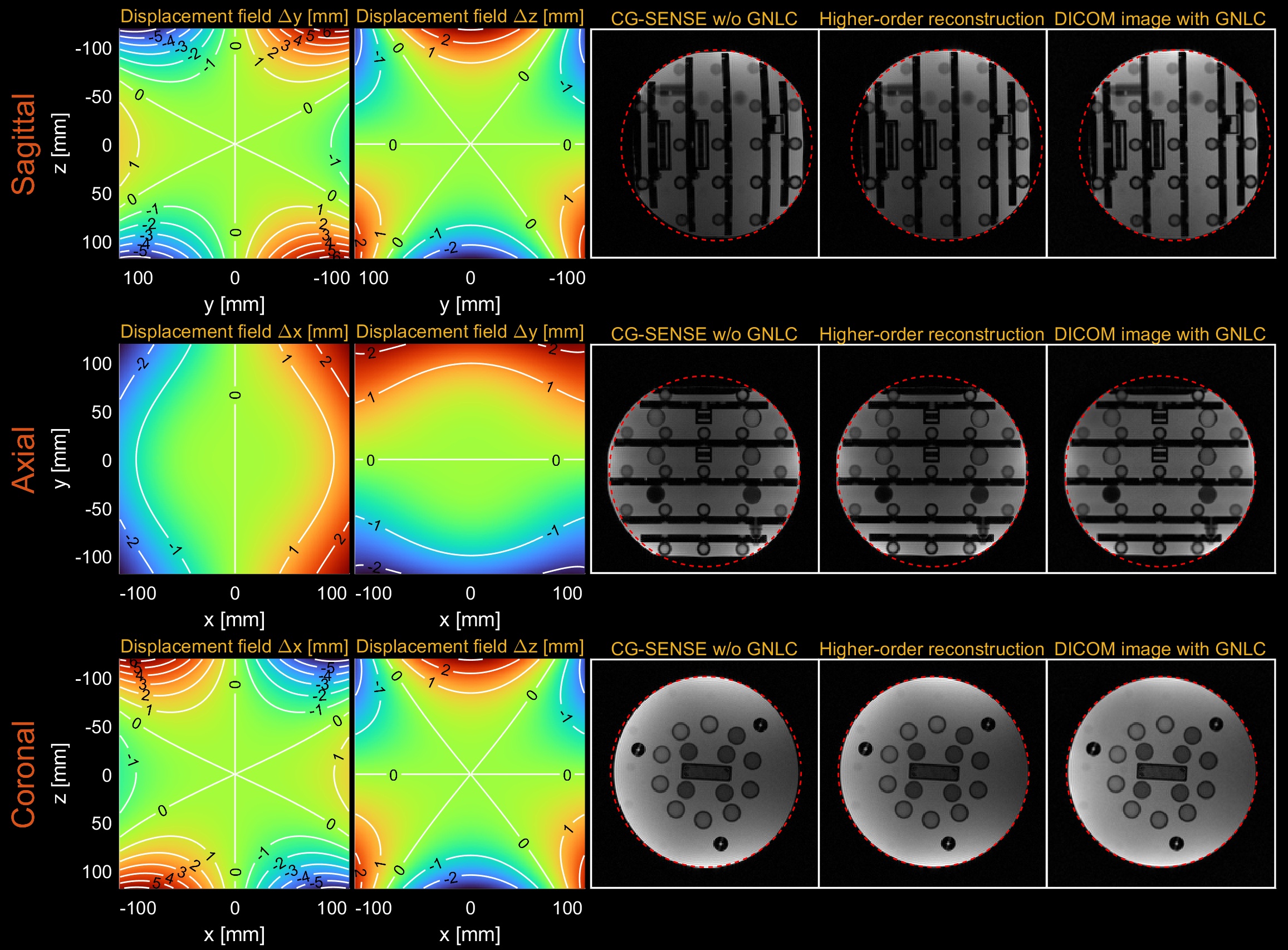
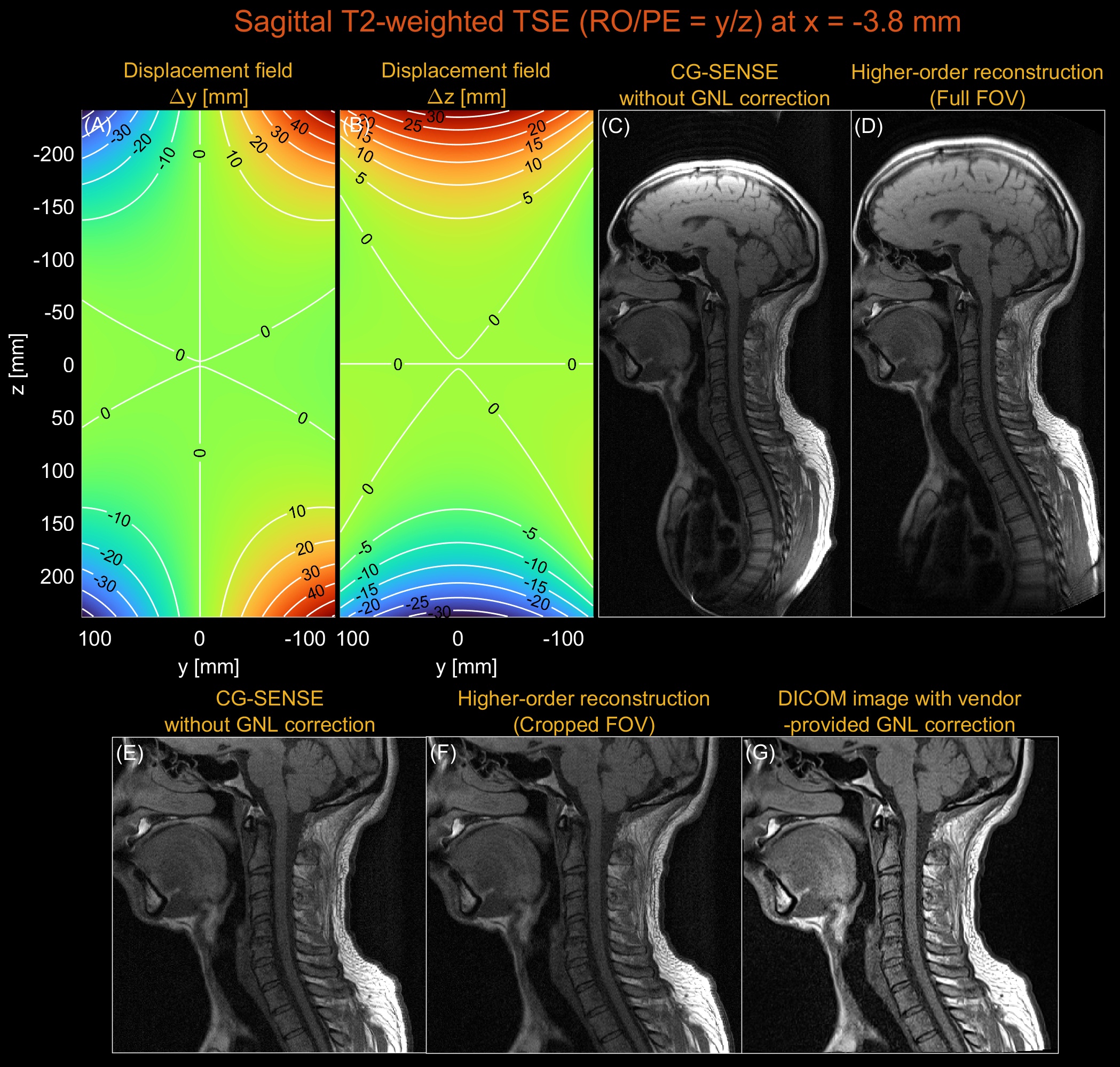
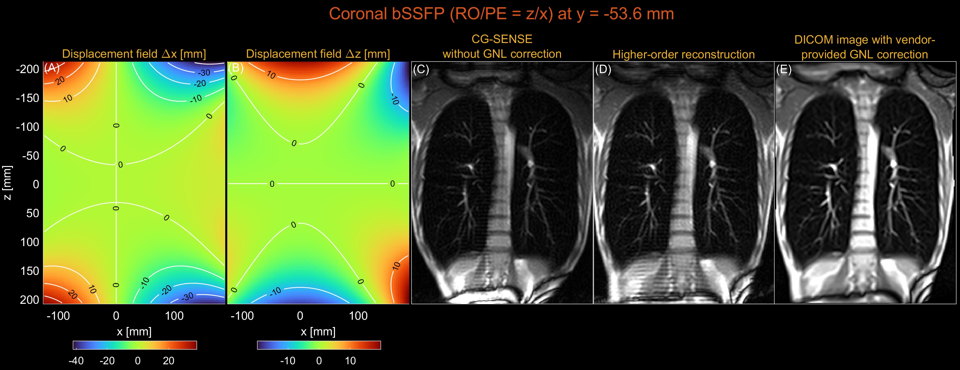
Figure 4. Gradient nonlinearity correction by higher-order reconstruction for a coronal Cartesian bSSFP scan. (A) Displacement field along the x-axis (PE). (B) Displacement field along the z-axis (RO). (C) CG-SENSE without GNL correction. (D) Higher-order image reconstruction (low-rank, L=80). (E) Vendor-provided GNL correction. Both GNL correction and surface coil intensity correction were applied to the DICOM image. Coil-combined images were first reconstructed, and zero-padding in k-space and cropping were performed to match the resolution and size of a DICOM image.