5011
Reconstruction May Benefit from Tailored Sampling Trajectories: Optimizing Non-Cartesian Trajectories for Model-based Reconstruction
Guanhua Wang1, Douglas C. Noll1, and Jeffrey A. Fessler2
1Biomedical Engineering, University of Michigan, Ann Arbor, MI, United States, 2EECS, University of Michigan, Ann Arbor, MI, United States
1Biomedical Engineering, University of Michigan, Ann Arbor, MI, United States, 2EECS, University of Michigan, Ann Arbor, MI, United States
Synopsis
This abstract explores non-Cartesian sampling trajectories that are optimized specifically for various reconstruction methods (CG-SENSE, penalized least-squares, compressed sensing, and unrolled neural networks). The learned sampling trajectories vary in the k-space coverage strategy and may reflect underlying characteristics of the corresponding reconstruction method. The reconstruction-specific sampling trajectory optimization leads to the most reconstruction quality improvement. This work demonstrates the potential benefit of jointly optimizing imaging protocols and downstream tasks (i.e., image reconstruction).
Introduction
For accelerated MRI, optimized sampling patterns can improve the image quality for a given acquisition time. Due to limited theories, MRI sampling pattern optimization often uses heuristics and grid search, such as variable density sampling [1]. By making the reconstruction method “differentiable” [2,3], this work used gradient-based methods to optimize sampling patterns w.r.t. reconstruction quality for several specific image reconstruction methods.We optimized trajectories with three types of reconstruction methods, namely smooth convex regularization (CG-SENSE, quadratic penalized least-squares (QPLS)), sparsity regularizer (compressed sensing, CS [4]), and model-based deep learning (MoDL [5]). Optimized trajectories exhibit different geometrical shapes and k-space coverage. Quantitative experiments show that the image quality benefited from the tailored sampling trajectory optimization.
Methods
For regularized MRI reconstruction, the cost function generally has the following form$$\hat{\boldsymbol{x}}=\underset{\boldsymbol{x}}{\arg \min }\|\boldsymbol{A} \boldsymbol{x}-\boldsymbol{y}\|_{2}^{2}+\mathsf{R}(\boldsymbol{x}).$$CG-SENSE uses a Tikhonov regularizer $$$\mathsf{R}(\boldsymbol{x})=\lambda\|\boldsymbol{x}\|_{2}^{2}.$$$
QPLS uses a finite-difference regularizer that encourages smoothness $$$\mathsf{R}(\boldsymbol{x})=\lambda\|\boldsymbol{D} \boldsymbol{x}\|_{2}^{2}.$$$
In compressed sensing, one regularizer option is an l1 norm of a discrete wavelet transform $$$\mathsf{R}(\boldsymbol{x})=\lambda\|\boldsymbol{W} \boldsymbol{x}\|_{1}.$$$
In unrolled neural networks, the optimization often alternates between two updates:$$\boldsymbol{z}_{i+1}=\mathcal{D}_{\boldsymbol{\theta}}\left(\boldsymbol{x}_{i+1}\right),$$ $$\boldsymbol{x}_{i+1}=\left(\boldsymbol{A}^{\prime} \boldsymbol{A}+\mu \boldsymbol{I}\right)^{-1}\left(\boldsymbol{A}^{\prime} \boldsymbol{y}+\mu \boldsymbol{z}_{i}\right).$$
Here, $$$\mathcal{D}_{\boldsymbol{\theta}}$$$ is a denoising/de-aliasing convolutional neural network [5]. In each case, the system matrix $$$A$$$ depends on the k-space sampling pattern $$$\boldsymbol{\omega}$$$, so the reconstructed image $$$\hat{\boldsymbol{x}}$$$ is also a function of the trajectory $$$\boldsymbol{\omega}$$$.
To optimize the sampling trajectories, this study used the loss function$$L(\boldsymbol{\omega})=\left\|\hat{\boldsymbol{x}}(\boldsymbol{\omega})-\boldsymbol{x}^{\text {true }}\right\|_{2}^{2},$$where $$$\boldsymbol{x}^{\text {true }}$$$ is the conjugate phase reconstruction of fully-sampled k-space. As is shown in Figure 1, the optimizer uses the negative of the loss gradient $$$\frac{\partial L}{\partial \boldsymbol{\omega}}$$$ to update trajectories [3].
Experiments
We used the fastMRI dataset [6] as the training set. The training process adopted the Adam optimizer with a learning rate = 1e-4, a batch size of 12, and 6 epochs. We also put a soft penalty on the maximum slew rate and gradient strength [2,7] (150 T/m/s, 50 mT/m). The initialization is a 16-spoke radial trajectory; each spoke is 5ms long with 1280 sampling points. To avoid sub-optimal local minimizers, we parameterized the sampling trajectories with 40 quadratic B-spline kernels [2]. Here we optimized a freeform non-Cartesian trajectory. Furthermore, the proposed method can also optimize parameters of predetermined geometrical shapes, such as the rotation angle of the radial trajectory.Results
Figure 2 showcases the optimized sampling trajectories for different reconstruction methods. The “density” of sampling points varies, especially in the center k-space. Figure 3 displays an example of reconstructed images. To investigate the transferability of learned trajectories, we reconstructed images with different methods using test data from each of the optimized trajectories. Table 1 displays the average quantitative reconstruction results on 500 test slices. The best results are when the trajectory is matched to the reconstruction method; the trajectory optimization can still improve the reconstruction quality with different reconstruction methods than that was used for training. Figure 3 displays examples of reconstructed images. Trajectory optimization results in reduced artifacts.Discussion
Via differentiable reconstruction and stochastic optimization, one may tailor sampling patterns for specific reconstruction methods. This work shows that different regularized reconstruction algorithms lead to distinct sampling trajectories, a trend that was also observed when optimizing Cartesian sampling [8]. This finding may encourage us to view acquisition and reconstruction as a unified problem.For simplicity, the current work uses the l2-norm as the loss function during training, which unavoidably focuses more on lower frequencies. In the future, we plan to use more advanced image quality metrics and possibly downstream tasks such as image segmentation as the training loss.
Acknowledgements
This work is supported in part by NIH Grants R01 EB023618 and U01 EB026977, and NSF Grant IIS 1838179.References
[1] Wang, Z., & Arce, G. R. (2009). Variable density compressed image sampling. IEEE Transactions on image processing, 19(1), 264-270.[2] Wang, G., Luo, T., Nielsen, J. F., Noll, D. C., & Fessler, J. A. (2021). B-spline parameterized joint optimization of reconstruction and k-space trajectories (bjork) for accelerated 2d mri. arXiv preprint arXiv:2101.11369.
[3] Wang, G. & Fessler, J. A. (2021). Efficient approximation of Jacobian matrices involving a non-uniform fast Fourier transform (NUFFT). arXiv preprint arXiv:2111.02912.
[4] Lustig, M., Donoho, D., & Pauly, J. M. (2007). Sparse MRI: The application of compressed sensing for rapid MR imaging. Magnetic Resonance in Medicine, 58(6), 1182-1195.
[5] Aggarwal, H. K., Mani, M. P., & Jacob, M. (2018). MoDL: Model-based deep learning architecture for inverse problems. IEEE transactions on medical imaging, 38(2), 394-405.
[6] Zbontar, J., Knoll, F., Sriram, A., Murrell, T., Huang, Z., Muckley, M. J., ... & Lui, Y. W. (2018). fastMRI: An open dataset and benchmarks for accelerated MRI. arXiv preprint arXiv:1811.08839.
[7] Weiss, T., Senouf, O., Vedula, S., Michailovich, O., Zibulevsky, M., & Bronstein, A. (2019). PILOT: Physics-Informed Learned Optimized Trajectories for Accelerated MRI. arXiv preprint arXiv:1909.05773.
[8] Zibetti, M. V., Herman, G. T., & Regatte, R. R. (2021). Fast data-driven learning of parallel MRI sampling patterns for large scale problems. Scientific Reports, 11(1), 1-19.
Figures
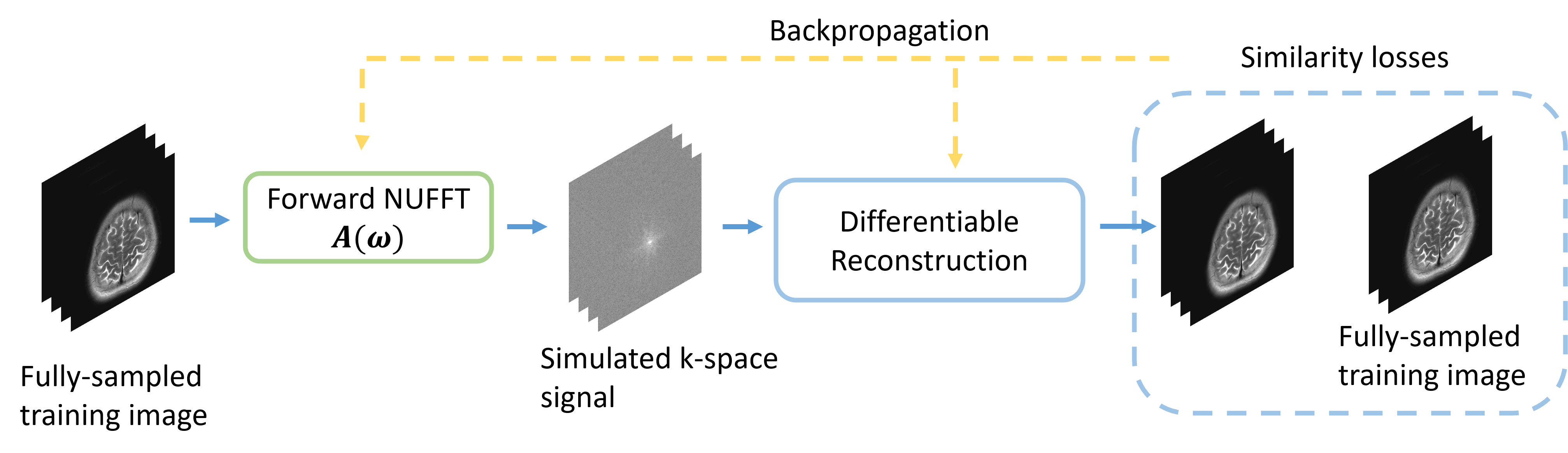
Figure 1. Diagram of the proposed stochastic optimization method. We used the chain rule to calculate the gradient of reconstruction loss with respect to the sampling trajectory.
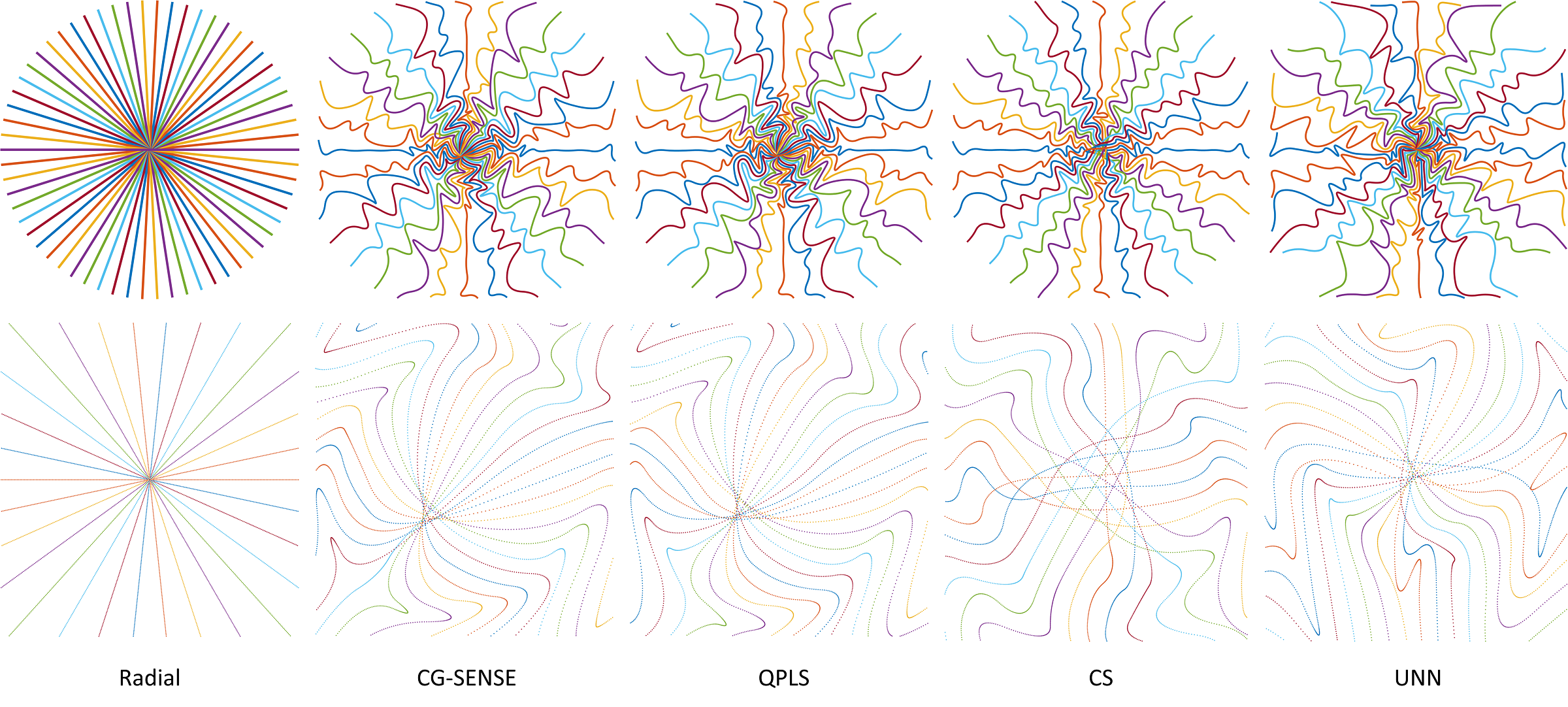
Figure 2. Optimized sampling trajectories for different reconstruction methods by gradient-based optimization. The second row shows the $$$8\times$$$ zoomed-in central k-space. The leftmost column shows the initialization of the trajectory optimization.
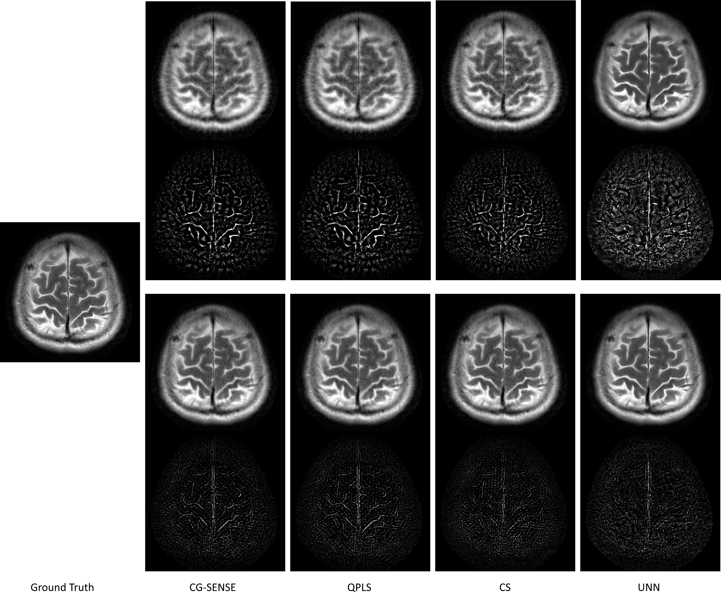
Figure 3. Examples of reconstructed test images with optimized trajectories by different methods. The first row shows the reconstructed images with the un-optimized trajectory, and the third row displays the results from optimized trajectories. The second and fourth row show the error maps, respectively.
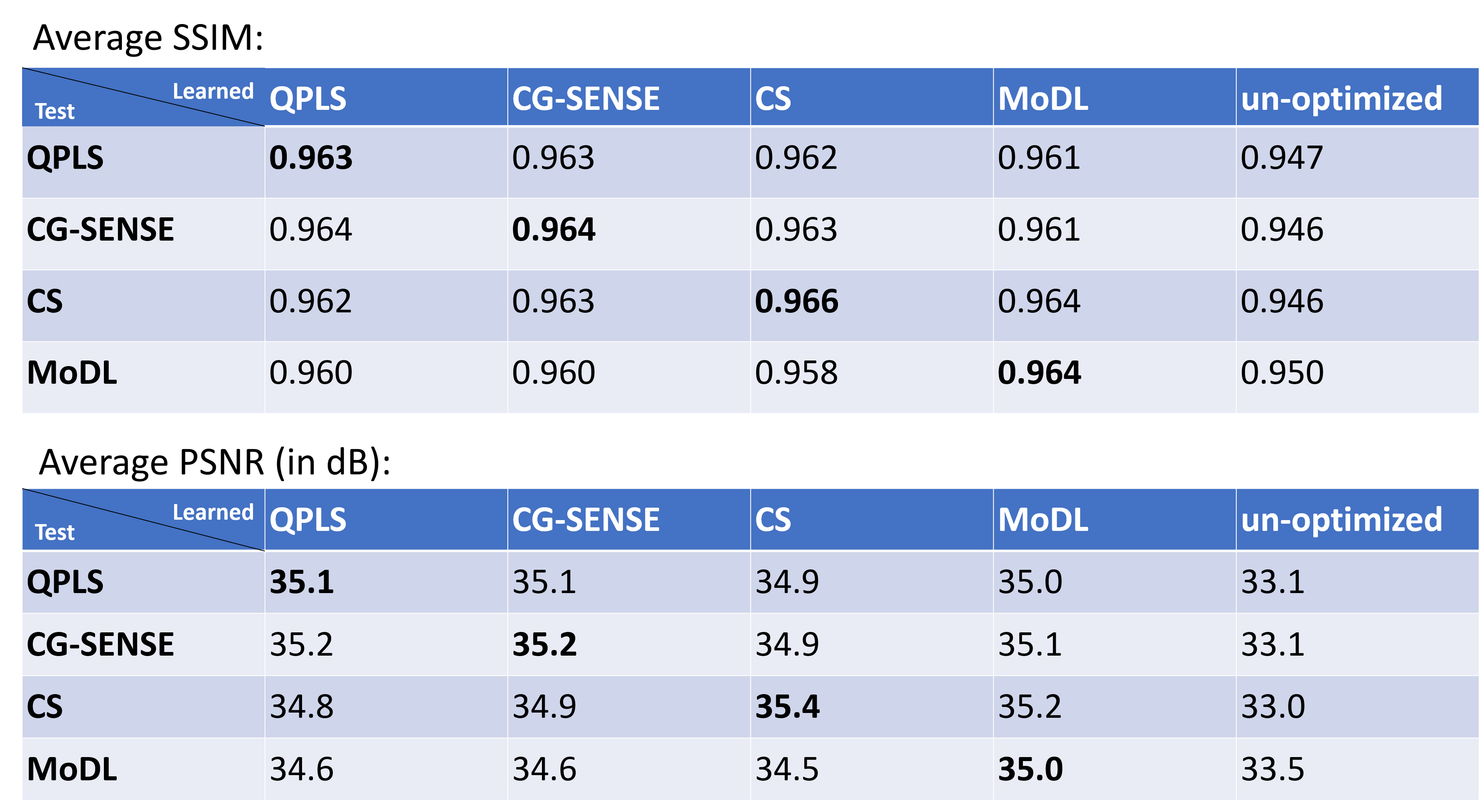
Table 1: The average quantitative reconstruction quality on the test set. The horizontal axis ('learned') stands for the sampling trajectory optimized with specific reconstruction methods. The vertical axis ('test') labels the reconstruction methods used for the test. The un-optimized label refers to the initialization (an undersampled radial trajectory).
DOI: https://doi.org/10.58530/2022/5011