5008
Acoustic Frequency Minimization of Gradient Waveforms with GrOpt1Radiology, Stanford University, Stanford, CA, United States, 2Radiology, Veterans Administration Health Care System, Palo Alto, CA, United States
Synopsis
In this work, we measured the acoustic frequency response function of an MRI scanner. The response was then used to design arbitrarily shaped gradient waveforms that minimize the predicted acoustic noise output of the sequence. Two minimization functions were tested and compared to the conventional sequence with two different slew rates. The method was used to generate a GRE sequence with 31% reduced acoustic output for a 17% increase in scan time or 16% reduced acoustic output compared to the slew rate derated sequence, both with no difference in image quality.
Introduction
High acoustic noise from MRI systems can lead to a patient anxiety and discomfort [1]. The primary source of this acoustic noise is from vibrations due to gradient coil activity, so designing pulse sequences to minimize noise can help with this problem.Previous work in the field of acoustic noise minimization has utilized lowpass filtering techniques to lower the spectral frequency of the acoustic noise where typical MRI systems usually have a weaker response [2]. Another proposed technique modifies gradient lobe timings relative to each other to avoid certain frequency ranges [3].
In this work, we aim to apply a numerically optimal design approach that acoustically minimizes the gradient waveforms while considering the entire frequency range and response of the MRI system. We do this by measuring the acoustic frequency response function [4,5] of a given MRI system, and then using an open source gradient optimization framework (GrOpt [6]) to design gradient waveforms that have a minimal predicted acoustic noise output based on the response function.
Methods
Frequency Response FunctionThe frequency response of the MRI system was measured by playing a series of short, different gradient waveforms subsequently on all three gradient axes. The audio from the sequence was measured with a microphone. Assuming a linear impulse response, we can describe the expected acoustic output: $$$a(t)=g(t)*h(t)$$$, where $$$g(t)$$$ is the gradient waveform and $$$h(t)$$$ is the acoustic impulse response. In the frequency domain this gives $$$A(f)=G(f)H(f)$$$ , where $$$H(f)$$$ is the desired acoustic frequency response function, which we obtained with an average of Weiner deconvolutions across all gradient pulses measured in the calibration scan.
Imaging Gradients and Optimization
A spoiled echo gradient sequence was designed using four different methods: (1) A traditionally “fast” waveform utilizing high slew rates (smax) and maximum gradient amplitude (gmax); and (2) A conventional “slow” sequence obtained by reducing the smax and gmax, with a corresponding increase in TE and TR (Figure 2). For (3) and (4), GrOpt was used to numerically optimize waveforms that minimized either (3) $$$\|W_A(f)G(f)\|_2$$$ or (4) $$$\|W_A(f)H(f)G(f)\|_2$$$, where is the standard A-weighting curve used in audio processing to account for the frequency dependent response of human perception to noise. (3) aims to use just A-weighting for minimization, which would not require measuring the acoustic response, while (4) uses the measured response functions (Hx,y,z) for each axis. The optimized sequences maintained the same gradient moments as the conventional sequences for all segments and gradient waveform timings matched to (2), the “slow” sequence.
Fig 2 shows gradient waveforms and parameters for the different sequences. Other parameters are: flip=10°, thickness=8mm, FOV=320x320, matrix=256x256. Sequences were all implemented in Pulseq [7].
Phantom Experiments and Analysis
The sequences were each run on a 3T Siemens Skyra scanner with a resolution phantom in a 32-channel chest coil. The audio was recorded during acquisition and the RMS average of the audio signal was reported after A-weighting in the frequency domain.
Results
Figure 1 shows the measured audio transfer functions (Hx,y,z). Figure 3 shows the gradient waveforms of the four different gradient configurations, along with the two frequency domain functions being minimized and their respective RMS norms. Figure 4 shows the images acquired with each of the GRE sequences, where little difference was seen in image quality. Figure 5 shows the recorded audio from each sequence in the frequency domain after A-weighting. The RMS average of each audio signal (arbitrarily scaled relative to the “slow” sequence) was: (1) 1.23, (2) 1.0, (3) 0.92, and (4) 0.84. For the full acoustic minimization sequence (fourth waveform), this represents a 31% decrease in acoustic noise compared to the fast scan, at the expense of a 17% increase in scan time, and a 16% reduction when compared to the conventional sequence with matched timings (“slow” waveforms).Discussion
This work showed that gradient waveform optimization can be used to control and minimize the frequency content of gradient waveforms and the predicted acoustic output of the scanner. By maintaining constraints on the required gradient moments and hardware limits of the system, there was no significant change in image quality. The gradient waveforms were in general more rounded, but with some high frequency components to give more time efficient encoding. When run on the scanner, the RMS power of the recorded audio was reduced by up to 16% with the optimized waveform, but not to the degree predicted analytically (50%). The discrepancy between analytical and experimental results may be attributed to a suboptimal measurement of the frequency response function (i.e. quality of the recording equipment used and selected calibration gradient waveforms). Future work will address this with improved microphone quality, and a longer and more robust calibration scan. Additionally, the optimization framework only optimizes individual TRs, without considering the inter-TR contributions to acoustic noise, which can be readily addressed with the same framework. The measured frequency response spectra were different for each gradient coil axes, which means that the acoustically minimized solution is rotationally variant. Another future area of interest for this work is in determining the ideal measure of acoustic loudness to optimize against [8].Acknowledgements
NIH Grant U01EB029427References
, , , 1989. Anxiety in patients undergoing MR imaging. Radiology;170:2:463–466.
[2] Hennel, F., Girard, F., Loenneker, T. (1999). "Silent" MRI with soft gradient pulses. Magnetic resonance in medicine, 42(1), 6–10.
[3] Segbers, M., Rizzo Sierra, C. V., Duifhuis, H., & Hoogduin, J. M. (2010). Shaping and timing gradient pulses to reduce MRI acoustic noise. Magnetic resonance in medicine, 64(2), 546–553.
[4] Hedeen, R. A., & Edelstein, W. A. (1997). Characterization and prediction of gradient acoustic noise in MR imagers. Magnetic resonance in medicine, 37(1), 7–10.
[5] Li, W., Mechefske, C., Gazdzinski C., Rutt, B. (2004), Acoustic noise analysis and prediction in a 4-T MRI scanner. Concepts Magn. Reson., 21B: 19-25.
[6] , , . A gradient optimization toolbox for general purpose time-optimal MRI gradient waveform design. Magn Reson Med. 2020; 84: 3234– 3245.
[7] Layton, K.J., Kroboth, S., Jia, F., Littin, S., Yu, H., Leupold, J., Nielsen, J.-F., Stöcker, T. and Zaitsev, M. (2017), Pulseq: A rapid and hardware-independent pulse sequence prototyping framework. Magn. Reson. Med., 77: 1544-1552.
[8] LUFS measurement from European Broadcasting Union standard ITU-R BS.1770
Figures
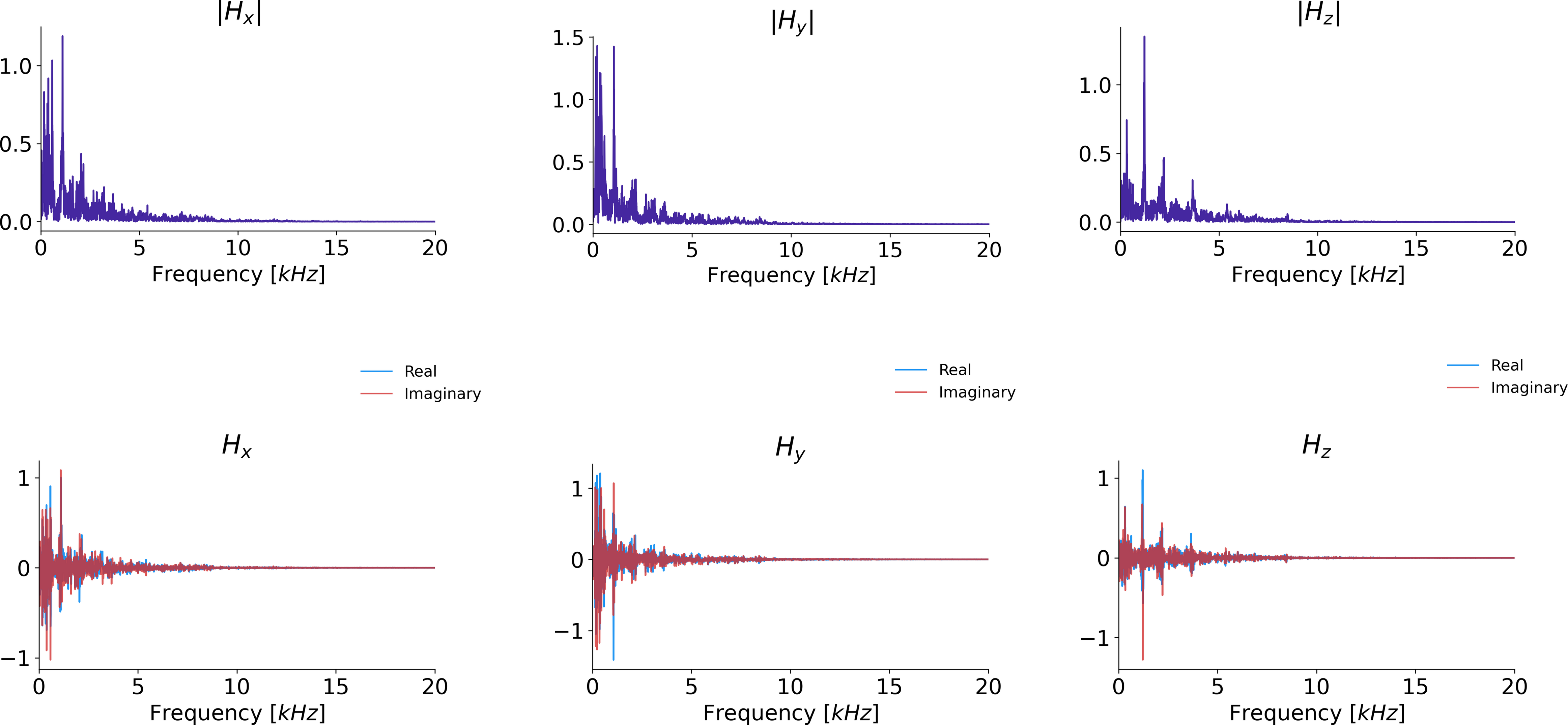
Figure 1: Measured acoustic frequency response functions for each gradient axis, y-axis units are arbitrary and linearly scaled. Top row shows the absolute value of the functions, and bottom row shows the complex values.
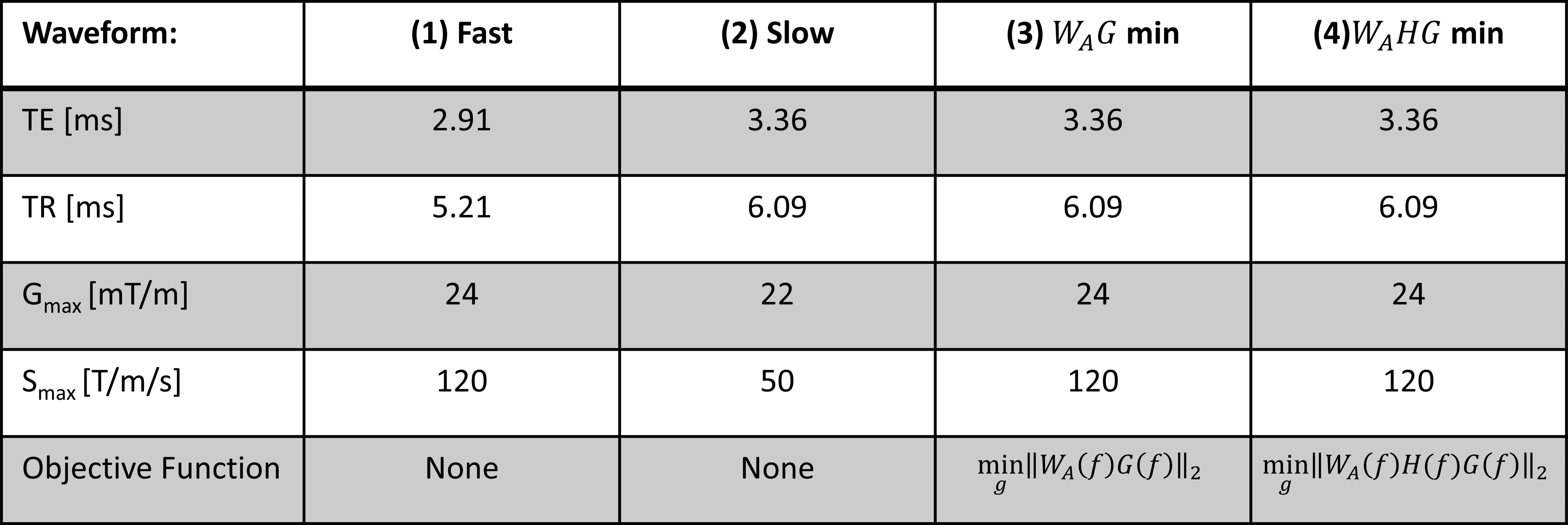
Figure 2: Table showing the most relevant scan parameter differences in waveforms between the 4 scans, and the objective functions minimized with GrOpt. The first two sequences represent conventional waveform design, where the shortest timings are found given the hardware and imaging constraints. The 3rd and 4th waveforms are optimized using the same timings as the conventional “slow” sequence, but utilizing the full hardware constraints to try to better minimize the objective functions.
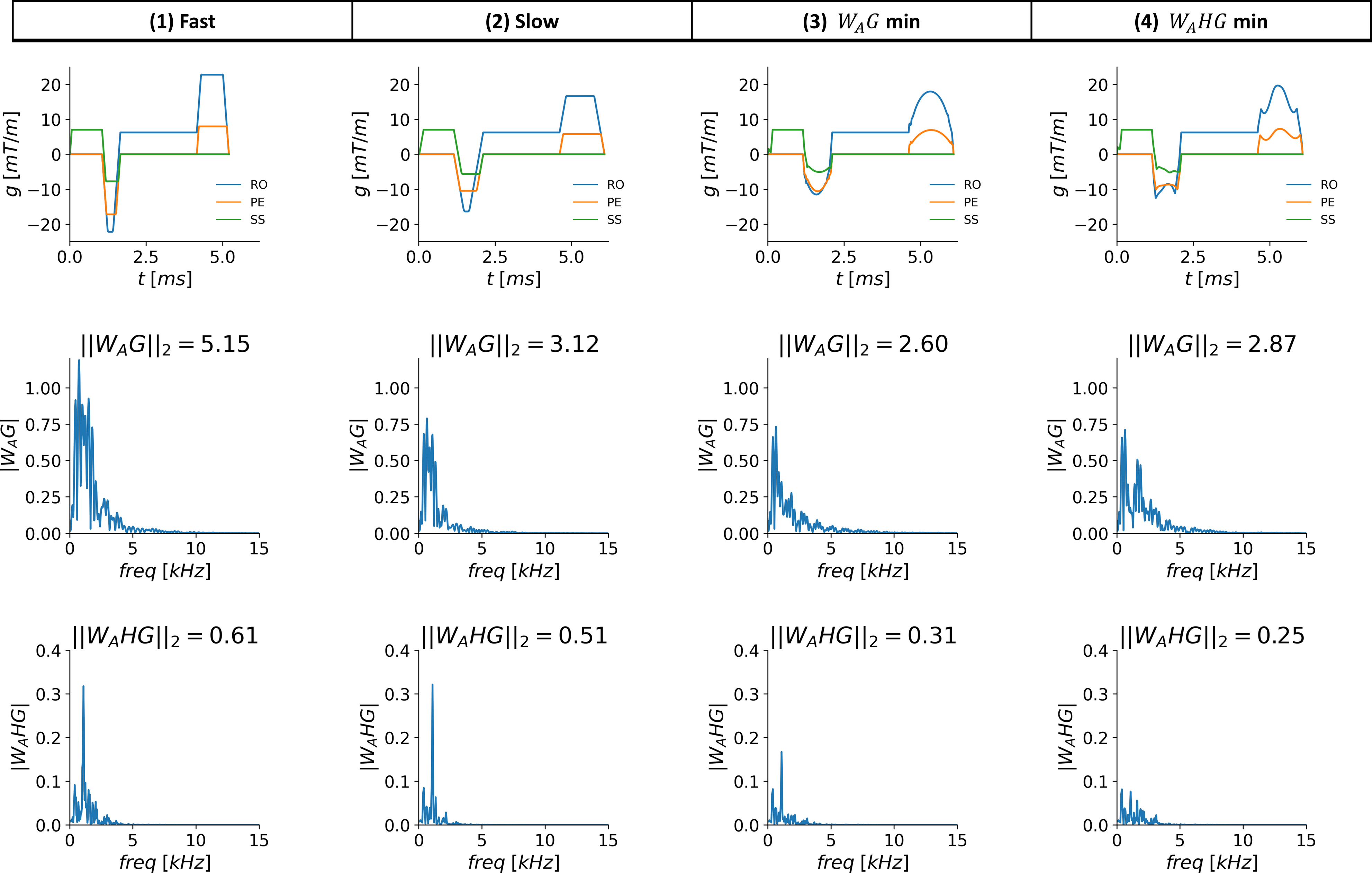
Figure 3: The four GRE pulse sequences used in this work (columns). The top row of plots shows all gradient waveforms for an example TR. The second row of plots shows the A-weighted frequency spectrum of the gradient waveform, which is the function being minimized with sequence 3. Hence, the lowest norm (||WAG||2) for this function is seen for sequence 3. Similarly, the last row shows the objective function with H(f) included. Hence, the lowest norm for this function is seen for sequence 4.

Figure 4: Reconstructed images from the 4 different acquisitions. Image quality differences are not apparent.

Figure 5: Frequency spectra of the recorded audio from the 4 different sequences. Y-axis has arbitrary units, with the same scaling between sequences.