5006
Quality Assessment of Mouse fMRI: Evaluating Temporal Stability of Preclinical Scanners1Biological & Biomedical Engineering, McGill University, Montreal, QC, Canada, 2Douglas Mental Health University Institute, Montreal, QC, Canada, 3Department of Psychiatry, McGill University, Montreal, QC, Canada
Synopsis
Mouse functional magnetic resonance imaging (fMRI) has interesting potential for basic neuroscience, but there is significant variability in data quality across studies. This variability may be partly explained by differences in scanner stability, however there are no reports of scanner quality assessments in the mouse fMRI field. We evaluated the stability of our preclinical scanner by acquiring an fMRI time-series of an agarose phantom then computing stability metrics. We found that our scanner has acceptable temporal stability but unexpected periodic fluctuations. Our methods are openly available so that other groups can easily implement stability assessments on their respective preclinical scanners.
Introduction
The aim of functional magnetic resonance imaging (fMRI) is to monitor fluctuations in neural activity, but in reality, most of the variance in the measured signal comes from fluctuations caused by motion, physiology and noise from the scanner itself. In the field of human fMRI, there have been efforts to minimize all the aforementioned sources of variance, including the implementation of regular assessments of scanner stability1-6. These scanner quality assessments (QA)s are crucial for identifying faulty equipment1, reducing variability between sites or timepoints3, and overall improving data quality7. In contrast, mouse fMRI literature focuses primarily on physiological confounds8, with no studies mentioning attempts to even evaluate the presence of scanner instabilities. Thus, we present a temporal QA protocol for preclinical scanners that includes: a) a recipe for creating a phantom with similar properties as the mouse brain and b) open-source code for automated analysis of a fMRI time-series acquired using the phantom. For the first time, we evaluate the temporal stability of the Bruker preclinical scanner. These results will notify other mouse fMRI groups of potential common issues with the Bruker scanner, and serve as a baseline for other centers to compare their results with.Methods
An agar phantom was constructed from 0.9% sodium chloride solution, agarose powder (2% w/v) and sodium azide (0.1% w/v)9. The mixture was doped with manganese chloride (0.0002% v/v; 1M solution) to obtain a T2* time of 43ms, approximately similar to that of the mouse brain.The phantom was scanned on a 7.0-T preclinical scanner (Bruker Biospec 70/30 USR; 30-cm inner bore diameter), equipped with a helium-cooled cryogenic surface transmit/receive coil (CryoProbeTM) as well as a room-temperature coil (volume transmitter, 4-channel array receiver). We acquired scans with both the cryogenic and room-temperature coils. A standard mouse fMRI gradient-echo echo planar imaging (GE-EPI) sequence was used: TR = 1000ms, TE = 15ms, matrix = 75x40, in-plane resolution = 0.25x0.25mm, slices = 26 interleaved, slice thickness = 0.5mm, bandwidth = 300480 Hz, 360 repetitions.
The data from the phantom fMRI scan was analyzed using a tailored pipeline made available online (https://github.com/CoBrALab/fMRI_phantom_analysis). First, the residuals were extracted by detrending the phantom time-series with a second order polynomial. We then computed standard scanner QA measures within each voxel: mean signal across time (before detrending), temporal fluctuation noise (standard deviation of the residuals across time), signal-to-fluctuation-noise ratio (mean signal divided by temporal fluctuation noise), static spatial noise (difference between sum of even images and sum of odd images). Additional metrics were computed within a region of interest (ROI): drift (change in the mean signal over time), percent fluctuation (standard deviation of the residuals divided by the mean), and radius of decorrelation (width of ROI at which statistical independence between voxels is lost)1,6. Finally, we incorporated a temporal principal components analysis (PCA) to decompose the data into orthogonal components that explain the most variance across time. Examining the temporal and spatial patterns of the PCA components is useful for diagnosing the causes of undesired, structured confounds; making our pipeline especially helpful for MRI technicians.
Results
Analysis of the phantom fMRI data revealed fluctuations in the signal over time. As the phantom is inanimate, the sole source of changes must be the scanner itself. Spatial maps of the mean signal, temporal fluctuation noise, signal-to-fluctuation-noise ratio (SFNR) and static spatial noise did not reveal any unusual patterns (figure 1). The drift, percent fluctuation and radius of decorrelation obtained with the CryoProbeTM were comparable to values from clinical scanners1,3, whereas the room-temperature coil performed worse (figure 2). Importantly, the percent fluctuation due to the scanner is much smaller than the expected percent changes in blood-oxygenation level dependent (BOLD) signal10.However, the PCA displayed unexpected results: there were two sinusoidal components with a frequency of 0.25 Hz (figure 3b,c), whose cause was identified as the IECO gradient amplifiers. As such, the characteristic frequency of these components changes unpredictably with the TR, number of slices and slice-encoding direction. Additionally, data acquired with the CryoProbeTM contained a slowly varying component that was not present in data from the room-temperature coil (figure 3a). The slow changes might be an effect of the CryoProbeTM’s external temperature settings, but we are still investigating the exact cause.
Discussion
Overall, our preclinical scanner was of satisfactory temporal stability and is suitable for monitoring fluctuations in the BOLD signal during mouse fMRI. We did, however, identify aspects of the preclinical scanner equipment that impact the fMRI signal; namely a periodic contribution from the gradient amplifiers and a slow non-linear trend in voxels next to the CryoProbeTM. Both of these contributions are relatively small, but it is nevertheless useful to be aware of them, as this knowledge can guide analysis choices and interpretation of results (for example: independent component analysis would be a better choice than a connectivity matrix given that the periodic confound has a non-homogenous spatial pattern). It is recommended for all mouse fMRI groups to perform a scanner QA before beginning a study; as it may identify issues that would otherwise corrupt the data, unnoticed.Acknowledgements
Thank you to the Fonds de Recherche du Quebec - Sante (FRQS) for funding this work. Thanks to Gabriel Devenyi and Gabriel Desrosiers-Gregoire for critical feedback.References
Friedman, L., & Glover, G. 2006. “Report on a Multicenter fMRI Quality Assurance Protocol.” Journal of Magnetic Resonance Imaging: JMRI 23 (6): 827–39.
Greve, D., Mueller, B., et al. 2011. “A Novel Method for Quantifying Scanner Instability in fMRI.” Magnetic Resonance in Medicine 65 (4): 1053–61.
Kayvanrad, A., Arnott, S., et al. 2021. “Resting State fMRI Scanner Instabilities Revealed by Longitudinal Phantom Scans in a Multi-Center Study.” NeuroImage 237 (August): 118197.
Simmons, A., Moore, E., and Williams, S. 1999. “Quality Control for Functional Magnetic Resonance Imaging Using Automated Data Analysis and Shewhart Charting.” Magnetic Resonance in Medicine 41 (6): 1274–78.
Smith, A. M., Lewis, B. K., et al. 1999. “Investigation of Low Frequency Drift in fMRI Signal.” NeuroImage 9 (5): 526–33.
Weisskoff, R. M. 1996. “Simple Measurement of Scanner Stability for Functional NMR Imaging of Activation in the Brain.” Magnetic Resonance in Medicine 36 (4): 643–45.
Lu, W., Dong, K., Cui, D., Jiao, Q., and Qiu, J. 2019. “Quality Assurance of Human Functional Magnetic Resonance Imaging: A Literature Review.” Quantitative Imaging in Medicine and Surgery 9 (6): 1147–62.
Mandino, F., Cerri, D.,et al. 2019. “Animal Functional Magnetic Resonance Imaging: Trends and Path Toward Standardization.” Frontiers in Neuroinformatics 13: 78.
Glover, G. 2005. “FBIRN Stability Phantom QA Procedures.” (2009-09-27) [2012-09-01]. Http://www. Birncommunity. Org/tools-Catalog/function-Birn-Stability-Pshantom-Qa-Procedures. nitrc.org. https://www.nitrc.org/frs/download.php/275/%EE%80%80fBIRN%EE%80%81_phantom_qaProcedures.pdf.
Desai, M., I. Kahn, U. Knoblich, J. Bernstein, H. Atallah, A. Yang, N. Kopell, et al. 2011. “Mapping Brain Networks in Awake Mice Using Combined Optical Neural Control and fMRI.” Journal of Neurophysiology 105 (3): 1393–1405.
Figures

Figure 1. Spatial maps of the mean signal across time, temporal fluctuation noise, signal-to-fluctuation-noise ratio (SFNR) and static spatial noise. Shown is a single slice through the center of the cylindrical phantom. The figure was generated with the open, custom analysis pipeline. A) Results from data acquired with the CryoProbe. B) Results from data acquired with the room-temperature coils. The mean signal is lower compared to the CryoProbe whereas the temporal fluctuation noise is greater. This effect is due to the higher thermal noise in the room-temperature coils.
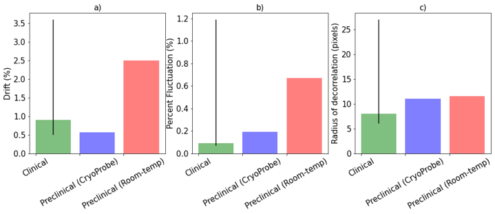

Figure 3. Each row shows the time series, Fourier spectrum and spatial pattern of a component from temporal PCA performed on data from the CryoProbe. The components shown are the top 6 that explain the most variance, in descending order. The colors of the spatial maps represent how strongly weighed that component is in each voxel. The figure was generated with the open, custom analysis pipeline. Component a) has a slowly-varying time series present in voxels next to the coil while components b,c are sinusoidal with a frequency of 0.25 Hz (red arrows) and have an inhomogenous spatial pattern.