Introduction

Balanced steady state free precession (bSSFP) is an SNR-efficient imaging modality with high fluid-tissue contrast, but the potential of the bSSFP sequence for quantitative tissue and environment parameter mapping is unrealized. bSSFP signal geometry is described by the elliptical signal model (ESM), which inspires analytical computations of ESM parameters. Previously, the geometric solution using 4 phase-cycled bSSFP images demonstrated the ability to generate artifact-free images and an off-resonance field map, with improved accuracy and SNR when combined with the algebraic solution.
Our work from last year attempted analytical computation of other bSSFP ESM parameters, leading to the first analytical $$$T_2$$$ computation based on the sum of squares (SOS) of four solutions. However, accuracy at large $$$T_2$$$ values was hindered by the required inverse logarithm. Rather than arbitrarily applying the SOS method that ignores each component’s relative veracity, an optimally weighted average (OWA) can leverage strengths and diminish weakness among different solutions. Here the refined analytical computation of $$$T_2$$$ relaxation using bSSFP ESM is formulated via a multi-step regional variance weighting method.

Theory

Eq.(1) describes the ESM for bSSFP signal, where the ESM parameters $$$|M|,a,b$$$ are defined in Eq.(2) with the equilibrium magnetization $$$M_0$$$, flip angle $$$\alpha,\,TR$$$, and relaxation times $$$T_1$$$ and $$$T_2$$$. Here $$$\theta$$$ and $$$\varphi$$$ respectively represent off-resonant phase accumulation at repetition time TR and echo time TE. $$$\psi$$$ is the phase cycling increment.
$$I(\theta,\psi)=M\frac{1-ae^{i(\theta+\psi)}}{1-b\cos(\theta+\psi)}e^{i\varphi}$$
$$\begin{aligned}E_{1}&:=\exp\left(-T R / T_{1}\right)\\E_{2}&:=\exp\left(-TR/T_{2}\right)\\a&:=E_{2}\\|M|&:=\frac{M_{0}\left(1-E_{1}\right)\sin\alpha}{1-E_{1}\cos\alpha-E_{2}^{2}\left(E_{1}-\cos\alpha\right)}\\b:&=\frac{E_{2}\left(1-E_{1}\right)(1+\cos\alpha)}{1-E_{1}\cos\alpha-E_{2}^{2}\left(E_{1}-\cos\alpha\right)}\end{aligned},(2)$$
Four unique datasets are considered with phase cycling increments $$$\psi_{1}=0^{\circ},\psi_{2}=90^{\circ},\psi_{3}=180^{\circ},\psi_{4}=270^{\circ}$$$ respectively.
As illustrated in our previous work, the geometric calculation of $$$b\cos\theta$$$ and $$$b\sin\theta$$$ can be found from the distances $$$d_{i}$$$ between the signal points $$$I_{i}=I\left(\theta,\psi_{i}\right)$$$ and the geometric solution crosspoint $$$M$$$,
$$\begin{gathered}d_{i}:=\left|I_{i}-Me^{i \varphi}\right|\\b\cos \theta=\frac{d_{1}-d_{3}}{d_{1}+d_{3}},b\sin\theta=\frac{d_{4}-d_{2}}{d_{2}+d_{4}},(3)\end{gathered}$$
This enables the transformation of the elliptical signal $$$I$$$ through multiplication by $$$(1\pm b\cos\theta)$$$ or $$$(1\pm b\sin\theta)$$$ to data on a "J-circle":
$$J(\theta,\psi)=I(\theta,\psi)(1-b\cos(\theta+\psi))=|M|e^{i\varphi}\left(1-ae^{i(\theta+\psi)}\right)$$
as shown in Fig.1.
Algebraic manipulation and uniform rotation of the J-circle datapoints by $$$\varphi$$$ gives:
$$ae^{i(\theta+\psi)}=1-\frac{e^{-i\varphi}J(\theta,\psi)}{M},$$
which yields 4 solutions of $$$\overrightarrow{a_{i}}=\left((a\cos\theta)_{i},(a\sin\theta)_{i}\right),\,i=1,2,3,4$$$, each corresponding to a different original data point.
The OWA of two solutions $$$sol_{i},\,sol_{j}$$$ may be expressed using regional variance weighting
$$\begin{aligned}&sol_{i j}=sol_{i}\cdot w_{i}+sol_{j}\cdot w_{j}\\&w_{i}=\frac{V_{j}}{V_{i}+V_{j}},w_{j}=\frac{V_{i}}{V_{i}+V_{j}},(6)\end{aligned}$$
with weights defined by regional noise variances $$$V_{i}, V_{j}$$$, which are computed on the difference of the solutions $$$sol_{i}, \,sol_{j}$$$ from a ground truth estimated from the weighted average of $$$sol_{i},\,sol_{j}$$$.
The Total Relative Error (TRE) of each analytical solution $$$f_{i}(x, y)=a,T_2$$$ over all pixel values $$$x,y$$$ is computed by
$$TRE(f)=\frac{\sqrt{\sum_{x, y}\left[f_{i}(x, y)-f_{g}(x, y)\right]^{2}}}{\sum_{x, y} f_{g}(x, y)},(6)$$
with respect to the gold standard $$$f_g$$$.

Methods

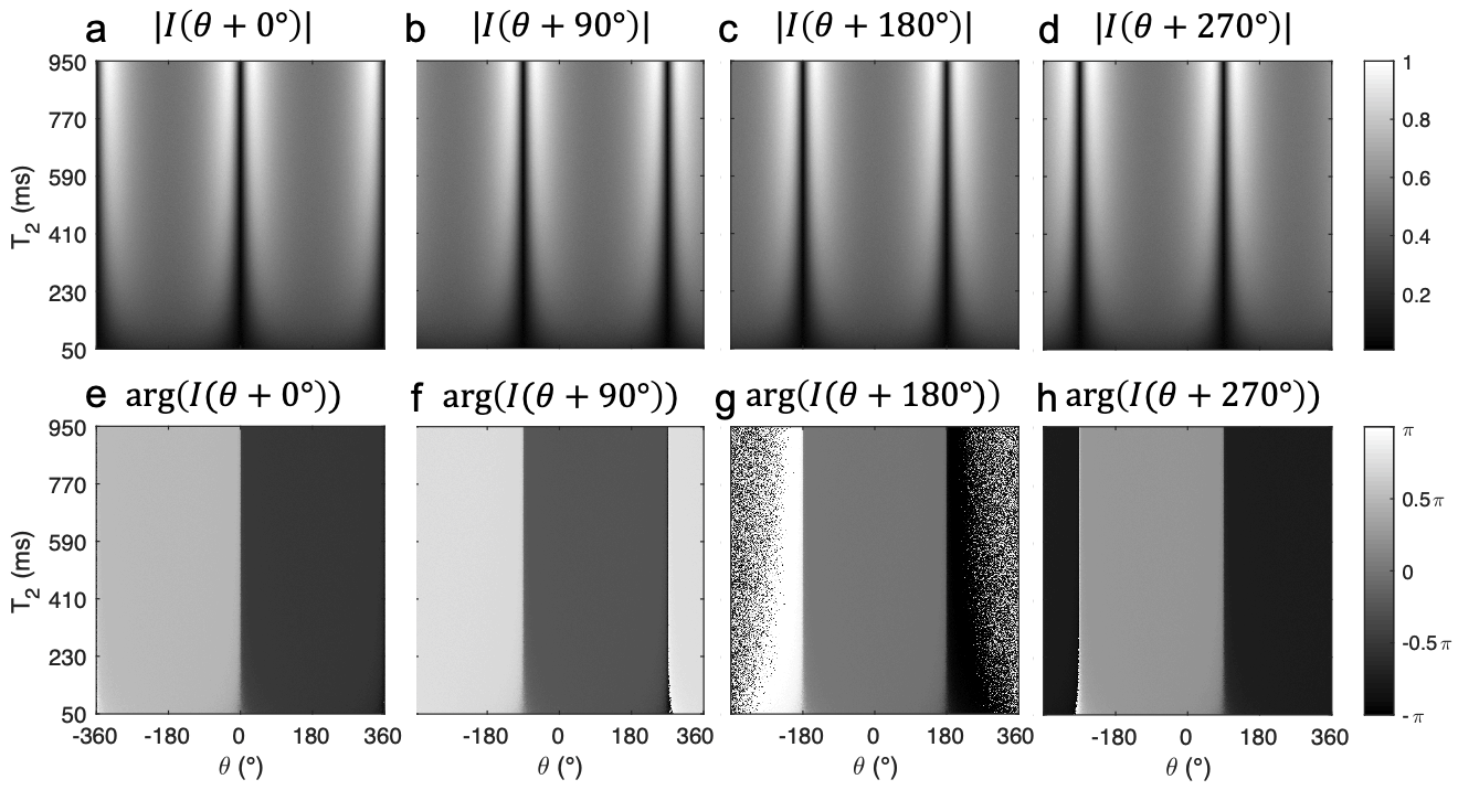
Four relatively phase-cycled images are simulated as described above, with flip angle $$$\alpha=30^{\circ}$$$ and $$$TR=10\mathrm{~ms}$$$. $$$T_{1}$$$ is held constant at $$$1000\mathrm{~ms}$$$. $$$T_{2}$$$ is uniformly varied from $$$50\mathrm{~ms}$$$ to $$$950\mathrm{~ms}$$$ vertically. The off-resonance angle $$$\theta$$$ varies from $$$-2\pi$$$ to $$$2\pi$$$ horizontally. Bivariate gaussian noise set to $$$2\%$$$ of the mean intensity is also added.
The solution of $$$b\cos\theta,b\sin\theta,\,\overrightarrow{a_{i}},\,i=1,2,3,4$$$ were computed pixelwise with signal real parts $$$x_{i}$$$, imaginary parts $$$y_{i}$$$ and the geometric solution cross-point $$$M=\left(M_{x},M_{y}\right)$$$.
The refined solution for $$$T_{2}$$$ is realized by a multi-step regional variance weighting
1.Optimally combine $$$\overrightarrow{a_{i}},\overrightarrow{a_{j}}$$$ for the $$$180^{\circ}$$$ phase-cycling pair $$$(i, j)=(1,3)\,\text{and}\,(2,4)$$$ to obtain $$$\overrightarrow{a_{13}}\,\text{and}\,\overrightarrow{a_{24}}$$$
2.Optimally combine $$$\overrightarrow{a_{13}}\,\text{and}\,\overrightarrow{a_{24}}$$$ to obtain $$$\overrightarrow{a_{(rv1)}}$$$ and hence $$$T_{2,(rv1)}=-TR/\ln\left|\overrightarrow{a_{(rv1)}}\right|$$$.
3.Optimally combine $$$T_{2,(13)}=-\mathrm{TR}/\ln\left|\overrightarrow{a_{13}}\right|$$$ and $$$T_{2,(24)}=-\mathrm{TR}/\ln\left|\overrightarrow{a_{24}}\right|$$$ to obtain another $$$T_{2}$$$ solution $$$T_{2,(rv2)}$$$.
4.Optimally combine $$$T_{2,(rv1)}\,\text{and}\,T_{2,(rv2)}$$$ to achieve the final solution $$$T_{2,(final)}$$$, which is analyzed later by computing TRE$$$\,\text{v.s.}\,T_{2},\theta$$$.
During the process, impossible $$$a geq1$$$ values corresponding to negative $$$T_{2}$$$ values are replaced with reasonable $$$a<1$$$ values based on regional averaging.

Results

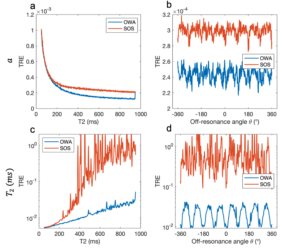
Fig.3 shows that the OWA method achieves lower error than the previously attempted SOS. Relative error is calculated and shown in the right column, indicating improved accuracy with band proximity and large $$$T_{2}$$$ values.
Fig.4 depicts the reduction of TRE of $$$a\,\text{and}\,T_{2}$$$ by the optimal weighted-sum method as a function of $$$T_{2}$$$ value and off-resonance $$$\theta$$$. The TRE of $$$T_{2}$$$ is decreased by up to 2 orders of magnitude at large $$$T_{2}$$$ values, as shown in Fig.4c and Fig.4d, with a periodic dependency of $$$T_{2}$$$ TRE on the off-resonance angle $$$\theta$$$.

Discussion

An optimal weighted sum of four $$$T_{2}$$$ solutions is proposed, which improves the analytical $$$T_{2}$$$ computation accuracy using the bSSFP ESM.
The $$$a\,\text{and}\,T_{2}$$$ solutions are exact and without error in noiseless scenarios for both SOS and OWA method. With noise present, the OWA possesses less error in $$$a\,\text{and}\,T_{2}$$$ than the SOS, especially at large $$$T_{2}$$$ values. The multi-step approach to variance weighting proposed is specifically designed to leverage the symmetry of bSSFP ESM:
1.Noise analysis revealed that solutions $$$\overrightarrow{a_{i}},\,\overrightarrow{a_{j}}$$$ from each $$$180^{\circ}$$$ phase-cycling pair have joint dependence on noise directed along the cross-point $$$M$$$ to datapoints $$$I_{i},\,I_{j}$$$, inspiring the initial combination of the $$$180^{\circ}$$$ pair solutions.
2.The variance weighting before (step 2) and after (step 3) taking the inverse logarithm create relatively good performance at small and large $$$T_{2}$$$ respectively.
The noise analysis indicates that $$$\overrightarrow{a_{i}}$$$ solutions have varied $$$\theta$$$-dependences, leading to the periodic dependency of $$$T_{2}$$$ TRE on $$$\theta$$$.

The multi-step regional-variance-weighted sum for $$$T_{2}$$$ computation using the ESM of bSSFP is shown to increase $$$T_{2}$$$ computation performance relative to the SOS, especially near dark bands. This analytical $$$T_{2}$$$ mapping refinement further novel clinical applications of bSSFP imaging.

Acknowledgements

No acknowledgement found.