Introduction

Subject motion is a common source of image artifacts that can severely decrease image quality and preclude clinical diagnosis in certain patient cohorts. Data-driven retrospective motion correction methods^1–3 are promising alternatives to rescanning that can be readily applied to clinical protocols to salvage corrupted images. While these approaches depend on classical optimization algorithms, recent advances leverage deep learning⁴ to incorporate useful image priors to assist with the high-dimensional, nonlinear optimization problem. Although the inclusion of deep learning has been shown to improve convergence speed⁴, it remains unclear whether deep learning can enable image recovery from heavily corrupted data that would otherwise be unsalvageable. In this abstract, we assess the performance limit of classical joint motion & image estimation and investigate the role of deep learning in severe motion corruption cases.

Methods

CNN-Assisted Joint Motion and Image Estimation
The motion-corrupted signal encoding process can be modeled as follows⁵:
$$ s =E_{\theta} m + \eta \tag{1}$$
$$ E_{\theta} = UFC\theta \tag{2}$$
where $$$s$$$ is the MR signal, $$$m$$$ is the magnetization image, $$$\eta$$$ is Gaussian noise, $$$U$$$ is the k-space undersampling matrix, $$$F$$$ is the Fourier transform, $$$C$$$ denotes the coil sensitivity profiles, and $$$\theta$$$ is composed of a rotation and a translation operator.
Given only the motion-corrupted signal, data-driven retrospective motion correction⁴ carries out motion-compensated image reconstruction (Eq. 3) by jointly estimating $$$m$$$ and $$$\theta$$$. This can be done using a data consistency formulation (Eq. 4) through the implicit encoding of motion afforded by multi-coil acquisition³.
$$ \hat{m} = \arg\min_{m} || E_{\hat {\theta}} m- s ||^2 \tag{3}$$
$$\hat{\theta} = \arg\min_{\theta} || E_{\theta} \hat{m} - s ||^2 \tag{4}$$
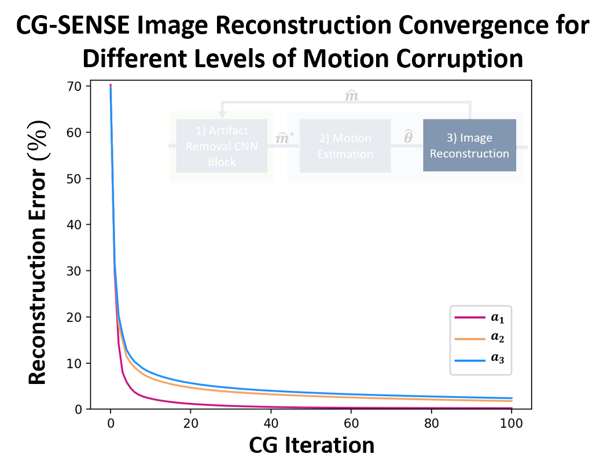
Eq. 3–4 are jointly estimated through coordinate gradient descent^3,4 using CG-SENSE⁶ and the BFGS optimization algorithm [7], respectively. The convergence of the joint estimation algorithm can be hindered by the coupling of $$$m$$$ and $$$\theta$$$ through the interdependence of Eq. 3 and 4⁴. A recent variant of the joint estimation framework (NAMER⁴), improved convergence behaviour by including a convolutional neural network (CNN) that was trained to estimate artifacts within a motion-corrupted input (Fig. 1). The estimated artifacts are subtracted to produce an artifact-reduced image (Eq. 5), which is then used in place of $$$\hat{m}$$$ in Eq. 4. We reimplemented the NAMER algorithm⁴ in Python using SigPy, CuPy, and TensorFlow.

$$\hat{m}^* = \hat{m} - CNN(\hat{m}) \tag{5}$$

Data
To facilitate reproducibility, simulations were conducted using a 2D slice of a T2w FSE brain MRI (3T Siemens, 0.49 mm isotropic in-plane resolution) and a motion trajectory provided by the authors of Reference 4 (max translation: $$$1.7 mm$$$; max rotation: 2.4 $$$2.4^\circ$$$). In-plane motion corruption was simulated using the signal encoding model (Eq. 1) with a $$$4x$$$- and $$$5x$$$- rescaling of the motion trajectory shown in Fig 2.a). and an R=2 Cartesian k-space undersampling pattern (Fig 2.b).

Assessing the Performance of Joint Estimation With and Without CNN
With the rescaled motion trajectories described above, we first investigated our baseline ability to reconstruct the uncorrupted image (Eq. 3) when provided with the groundtruth motion parameters.
Continuing with the same motion corruption cases, we compared the convergence behaviour of the joint estimation algorithm with and without the CNN. We analyzed the motion estimation optimization trajectory and assessed the impact of including the CNN.

Results

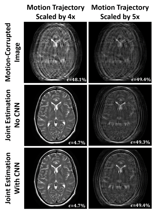
For all motion-corrupted data, the CG-SENSE algorithm was able to accurately recover the uncorrupted image when provided with the groundtruth motion parameters (Fig. 3). After 100 iterations, reconstructions errors of 1.8%, and 2.4% were achieved for the $$$4x$$$- and $$$5x$$$- rescaled motion trajectories. The number of CG-SENSE iterations required to reach convergence increased as motion severity increased.

In Fig. 4, we show the results of the outputs of the joint estimation algorithm (with and without the CNN) for the $$$4x$$$- and $$$5x$$$- rescaled motion trajectory. For the former case, the algorithm converged to an accurate estimate of the uncorrupted image ($$$\epsilon$$$) with and without the CNN (Fig. 4). For the latter case, the algorithm converged to images with significant residual motion artifacts with and without the CNN, resulting in no improvement in computed reconstruction error.

In Fig. 5, we show the corresponding motion estimation convergence curves for the results shown in Fig. 4. For the $$$4x$$$- rescaled case, we see that including the CNN resulted in faster convergence (by a factor of 1.8). For the $$$5x$$$- rescaled case, we see that motion estimation optimization has converged to suboptimal values with and without the CNN.

Discussion and Conclusions

Here, we presented results of joint estimation with and without the CNN under different examples of severe motion corruption. We had first confirmed that, given the groundtruth motion parameters, we could accurately recover the uncorrupted images (Fig. 3). As such, the differing reconstruction qualities demonstrated in Fig. 4 was due varying levels of success in estimating the motion parameters. This was confirmed by Fig. 5, where we additionally demonstrate the CNN’s potential to speed up convergence towards accurate motion parameter estimates, corroborating previous findings⁴. From our study, it appears that beyond convergence acceleration, the CNN was not able to salvage motion-corrupted images beyond the joint estimation’s principal capability. However, a more exhaustive study is required to corroborate this finding.

References

[1] D. Atkinson, D. L. G. Hill, P. N. R. Stoyle, P. E. Summers, and S. F. Keevil, “Automatic correction of motion artifacts in magnetic resonance images using an entropy focus criterion,” IEEE Trans. Med. Imaging, vol. 16, no. 6, pp. 903–910, 1997
[2] A. Loktyushin, H. Nickisch, R. Pohmann, and B. Schölkopf, “Blind retrospective motion correction of MR images,” Magn. Reson. Med., vol. 70, no. 6, pp. 1608–1618, 2013
[3] L. Cordero-Grande, R. P. A. G. Teixeira, E. J. Hughes, J. Hutter, A. N. Price, and J. V. Hajnal, “Sensitivity Encoding for Aligned Multishot Magnetic Resonance Reconstruction,” IEEE Trans. Comput. Imaging, vol. 2, no. 3, pp. 266–280, 2016
[4] M. W. Haskell et al., “Network Accelerated Motion Estimation and Reduction (NAMER): Convolutional neural network guided retrospective motion correction using a separable motion model,” Magn. Reson. Med., vol. 82, no. 4, pp. 1452–1461, 2019
[5] P. G. Batchelor, D. Atkinson, P. Irarrazaval, D. L. G. Hill, J. Hajnal, and D. Larkman, “Matrix description of general motion correction applied to multishot images,” Magn. Reson. Med., vol. 54, no. 5, pp. 1273–1280, 2005
[6K. P. Pruessmann, M. Weiger, M. B. Scheidegger, and P. Boesiger, “SENSE: Sensitivity encoding for fast MRI,” Magn. Reson. Med., vol. 42, no. 5, pp. 952–962, Nov. 1999
[7] J. Nocedal and S. J. Wright, Numerical optimization, 2nd ed. New York: Springer, 2006.
[8] L. Cordero‐Grande, G. Ferrazzi, R. P. A. G. Teixeira, J. O’Muircheartaigh, A. N. Price, and J. V. Hajnal, “Motion-corrected MRI with DISORDER: Distributed and incoherent sample orders for reconstruction deblurring using encoding redundancy,” Magn. Reson. Med., vol. 84, no. 2, pp. 713–726, 2020