4989
Increased repeatability in blind source separation analysis of dynamic contrast enhanced MRI1Medical Physics Unit, McGill University, Montreal, QC, Canada, 2Mayo Clinic, Rochester, MN, United States, 3Research Institute of the McGill University Health Centre, Montreal, QC, Canada
Synopsis
Blind source separation can be used to linearly decompose DCE-MRI time-course data into a sparse set of time courses, or sources, and maps of coefficients, or weights, to describe the entire 4D dataset. This type of analysis generates in realistic time-courses for the wash-in and wash-out of the contrast agent, and maps of the distribution of these dynamics. In turn, these decompositions may hold diagnostic value. Random initialization typical of such algorithms makes the output unstable. This work sought design an approach to blind source separation analysis of DCE-MRI with lower variability and independent of NMF initialization.
INTRODUCTION
Pattern recognition techniques based on blind source separation (BSS) can be used as a model-free approach to identify perfusion patterns in cancer tumours and form maps that reflect tumour heterogeneity1,2. BSS can decompose a set of mixed signals into separate source signals without a priori information on the source signals or the mixing process. Non-negative matrix factorization (NMF)3 is a well-known BSS approach that uses dimensionality reduction with visualization capabilities. NMF in DCE-MRI is plagued by non-uniqueness of the matrix factorization for a given dataset due to random initialization4. This work proposes “multi-run” NMF, or multiNMF, to address the non-uniqueness of NMF4,5 in analysis of DCE-MRI. The performance is demonstrated on data from patients with high grade soft tissue sarcoma6.METHODS
The multiNMF approach performs multiple runs of NMF on a given dataset and uses the mean of all weight maps produced as the most representative weight map of the patient dataset. To determine the number of runs required to obtain a representative mean weight map, a method was devised based on the variation of the mean when a new run is added to the averaging process. The Euclidian distance between successive mean weight maps is computed as a difference metric at each iteration and normalized by the number of pixels in the image. Additional runs of NMF are added to the running mean until the difference metric drops below a pre-set tolerance. The running mean weight map calculated during the process can be affected by solutions far from the mean, driven by the random initialization. A more stable running mean can be obtained by considering the ten most recent outputs (using a window of 10 individual runs of NMF). Finally, once the final mean weight map is computed, the sources that best fit the data can be recomputed using the appropriate decomposition step from the NMF algorithm with the original data.In this work, the ANLS-BPP algorithm7 was used as the core NMF method, set up a priori to identify two sources. A low number of sources enforces a sparse description of perfusion in tissue, and two sources were selected here as qualitatively enough to ensure a stable factorization.
Data were selected ad hoc from 8 of 18 patients with histologically proven high-grade soft-tissue sarcoma6. This dataset featured exams performed at 1.5 T, including DCE-MRI, over a course of neoadjuvant radiotherapy, acquired prospectively under institutional approval with informed consent. Only data from pre-treatment exams were used here. Dynamic T1-weighted time-series images were acquired during intravenous injection of gadobutrol (Gadovist, Bayer, 0.1 mmol/kg), using a 3D fast spoiled gradient echo sequence (number of frames ~ 45 and frame time = 10.2–14.4 s depending on the patient, TR=6.0 ms, TE=4.2 ms, flip angle=25°, matrix =256×128, and field-of-view = 24-28 cm). Manual contours of the sarcoma were produced by a radiation oncologist and used to include only the tumour in the analysis, excluding healthy tissue.
Test data for multiNMF were generated using the ANLS-BPP algorithm to create 1,000 distinct single runs from random initializations in the patient datasets. multiNMF was then applied retrospectively to these individual runs to generate up to 10 mean weight maps per data set, depending on the number of runs used in each multiNMF. Three tolerance levels were tested (0.01, 0.001, and 0.001). The variability of the NMF and multiNMF outputs were calculated from the standard deviation of the weight maps.
RESULTS
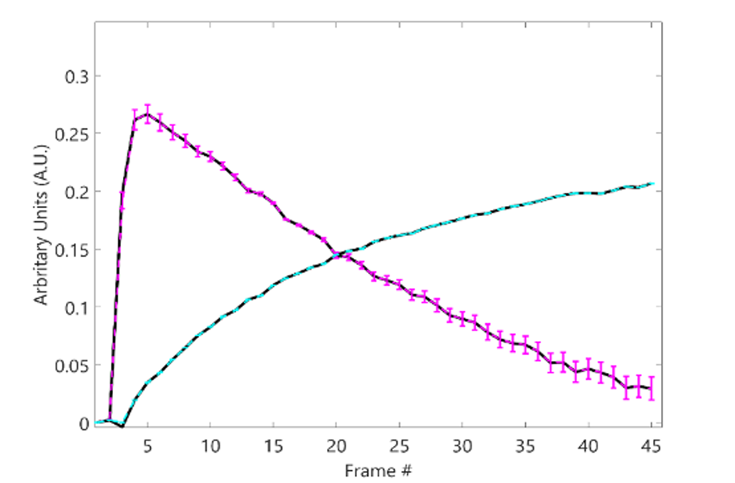
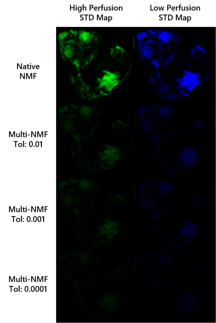
The multiNMF approach resulted in a reduction of the variability of weight maps, as illustrated for one patient dataset in Figure 1. Gains in repeatability were seen at all tolerances for the distance between successive averages, with decreases in the average standard deviation of at least a factor of 3 for the highest tolerance value (Figure 2). Reaching the tolerance of 0.01 typically require up to 10 runs of NMF, or around 1 minute of processing, which is largely justified to stabilize the output of the analysis. A tolerance of 0.0001 requires on the order of 100 runs (around 10 minutes). The source curves generated by multiNMF were identical to the average of curves from 1000 runs, confirming that the multiNMF trends towards the average behaviour (Figure 3).DISCUSSION AND CONCLUSION
The multiNMF algorithm improves on native NMF (ANLS-BPP here) by decreasing variability in the perfusion weight maps. Decreasing the tolerance in the multiNMF further reduces the variability of the perfusion weight maps but increases the processing time: the optimal tolerance is work in progress. multiNMF can nominally be applied to any NMF algorithm to reduce variability on the perfusion maps.A bootstrapping method previously proposed to address the non-uniqueness of NMF in DCE-MRI selects the most frequent solution 4 and would be interesting to compare. Other initialization techniques have been proposed for NMF algorithms applied DCE-MRI datasets. Data-driven initialization of the Block-coordinate Update NMF (BU-NMF) algorithm with wash-in or Ktrans maps, produced interpretable and repeatable results on data from patients with sarcomas2,8,9. Our approach reduces the variability without requiring a priori information such as the Ktrans maps (which would require T1 and B1 maps)
Acknowledgements
We acknowledge funding from NSERC and FRQS.
References
REFERENCES:
[1] R. Stoyanova et al., “Mapping Tumor Hypoxia In Vivo Using Pattern Recognition of Dynamic Contrast-enhanced MRI Data,” Translational Oncology, vol. 5, no. 6, pp. 437- IN2, 2012.
[2] M. Venianaki et al., “Pattern recognition and pharmacokinetic methods on DCE-MRI data for tumor hypoxia mapping in sarcoma,” Multimedia Tools and Applications, vol. 77, no. 8, pp. 9417–9439, 2018.
[3] D. D. Lee and H. S. Seung, “Learning the parts of objects by non-negative matrix factorization,” Nature, vol. 401, no. 6755, pp. 788–791, 1999.
[4] G. Casalino, N. Del Buono, and C. Mencar, “Nonnegative matrix factorizations for intelligent data analysis,” in Non-negative Matrix Factorization Techniques: Advances in Theory and Applications, Springer Berlin Heidelberg, 2015, pp. 49–74.
[5] E. Kontopodis et al., “Investigating the role of model-based and model-free imaging biomarkers as early predictors of neoadjuvant breast cancer therapy outcome,” IEEE Journal of Biomedical and Health Informatics, vol. 2194, no. c, pp. 1–1, 2019.
[6] M. Vallières et al., “Investigating the role of functional imaging in the management of soft- tissue sarcomas of the extremities,” Physics and Imaging in Radiation Oncology, vol. 6, no. April, pp. 53–60, 2018.
[7] J. Kim and H. Park, “Fast nonnegative matrix factorization: An active-set-like method and comparisons,” SIAM Journal on Scientific Computing, vol. 33, no. 6, pp. 3261–3281, 2011.
[8] M. Venianaki et al., “Improving hypoxia map estimation by using model-free classification techniques in DCE-MRI images,” IST 2016 - 2016 IEEE International Conference on Imaging Systems and Techniques, Proceedings, pp. 183–188, 2016.
[9] Y. Xu and W. Yin, “A Block Coordinate Descent Method for Regularized Multiconvex Optimization with Applications to Nonnegative Tensor Factorization and Completion,” SIAM Journal on Imaging Sciences, vol. 6, no. 3, pp. 1758–1789, 2013.
Figures
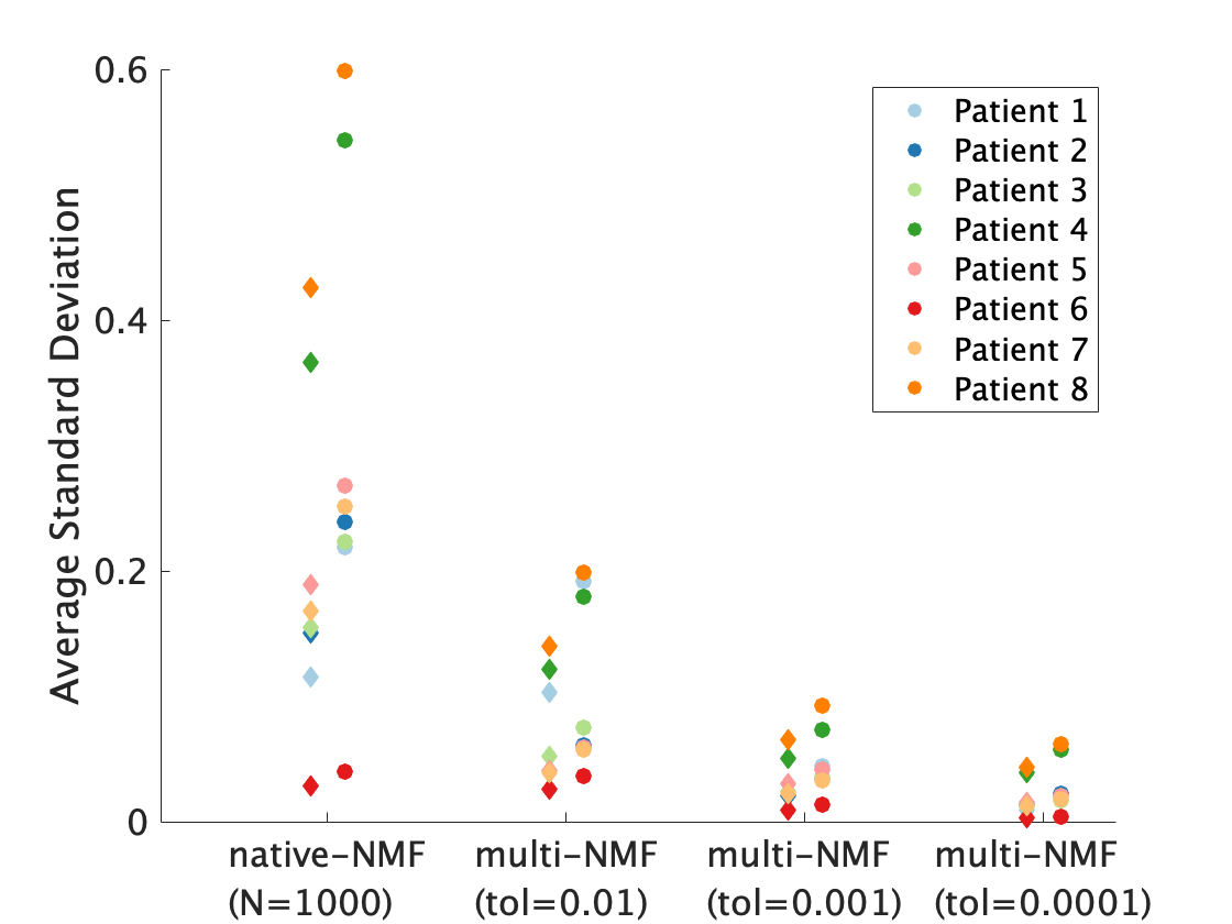
Mean of the standard deviation of voxel weights for native NMF (n=1000 runs) and multi-NMF for tolerance levels: 0.01, 0.001, 0.0001, for the 8 datasets. The high perfusion source weights are represented by the diamonds, and the low perfusion by the circles. In all patients, the overall standard deviation was reduced in multi-NMF compared to native-NMF and more so with lower tolerance.