4982
MIRTorch: A PyTorch-powered Differentiable Toolbox for Fast Image Reconstruction and Scan Protocol Optimization
Guanhua Wang1, Neel Shah2, Keyue Zhu2, Douglas C. Noll1, and Jeffrey A. Fessler2
1Biomedical Engineering, University of Michigan, Ann Arbor, MI, United States, 2EECS, University of Michigan, Ann Arbor, MI, United States
1Biomedical Engineering, University of Michigan, Ann Arbor, MI, United States, 2EECS, University of Michigan, Ann Arbor, MI, United States
Synopsis
MIRTorch (Michigan Image Reconstruction Toolbox for PyTorch) is an image reconstruction toolbox implemented with native Python/PyTorch. It provides fast iterative and data-driven image reconstruction on both CPUs and GPUs. Researchers can rapidly develop new model-based and learning-based methods (i.e., unrolled neural networks) with its convenient abstraction layers. With the full support of auto-differentiation, one may optimize imaging protocols, such as sampling patterns and image reconstruction parameters with gradient-based methods.
Inspiration
The rapid development of auto-differentiation toolchains brings our community new computation infrastructure. This abstract presents MIRTorch, which aims to use the speed and hardware adaptability of PyTorch. Researchers can run fast iterative reconstruction and quickly prototype novel methods. By the native support of auto-differentiation, the reconstruction methods are differentiable, thus can be easily merged into deep learning-based methods. By defining the quality of downstream tasks (such as reconstruction or segmentation) as the training loss, gradient-based methods can use backpropagation to optimize imaging protocols, such as RF pulses and readout trajectories.Design
Inspired by the MIRT [1], SigPy [2], and PyLops [3], the MIRTorch toolbox contains the following essential components:Linear operators
The package provides common image processing operations, such as convolution. For MRI reconstruction, the system matrices include Cartesian and Non-Cartesian, and coil sensitivity- and B0- informed models. Since the Jacobian matrix of a linear operator is itself, the toolbox may actively calculate such Jacobians during backpropagation instead of the auto-differentiation approach, avoiding the enormous cache cost.
Proximal operators
The toolbox contains common proximal operators such as soft thresholding. These operators also support regularizers that involve multiplication with diagonal or unitary matrices, such as orthogonal wavelets.
Optimization algorithms
The package includes the conjugate gradient (CG), FISTA [4], POGM [5], PDHG [6], and ADMM [7] algorithms for image reconstruction.
Dictionary learning:
For dictionary learning-based reconstruction, we implemented an efficient dictionary learning algorithm (SOUP-DIL [8]) and orthogonal matching pursuit (OMP [9]). Due to PyTorch’s limited support of sparse matrices, we use SciPy as the backend.
Usage
Iterative reconstructionFor model-based MRI reconstruction, the cost function usually has this form
$$\hat{\boldsymbol{x}}=\underset{\boldsymbol{x}}{\arg \min }\|\boldsymbol{A} \boldsymbol{x}-\boldsymbol{y}\|_{2}^{2}+\mathsf{R}(\boldsymbol{x}).$$To build a user-defined reconstruction method, one should define a system matrix $$$\boldsymbol{A}$$$, regularizer $$$\mathsf{R}(\cdot)$$$ and choose a corresponding optimization algorithm. If $$$\mathsf{R}(\cdot)$$$ is smooth and convex, one may consider using basic gradient descent (GD) or the optimized gradient method (OGM [10]) to solve it. If $$$\mathsf{R}(\cdot)$$$ is proximal-friendly, one may use FISTA or POGM. Otherwise, one can use ADMM or PDHG as the optimization algorithm, if applicable.
Model-based deep learning
With MIRTorch, researchers can also easily define new instances of unrolled neural networks.For example, one can build a MoDL model [11] in a few lines:
A = Sense(sensemap, mask)
I = Identity(A.size_in)
CG_solver = CG(A.H*A + lamda * I)
for i in range(num_iter):
z_i = self.netD(x_i)
x_i = CG_solver(z_i, A.H*self.kdata +lamda*z_i)
Examples
We illustrate several reconstruction methods with Jupyter Notebooks, including (B0-informed) penalized least-squares reconstruction, dictionary learning reconstruction [8], compressed sensing reconstruction (CS, [12]), and unrolled neural network-based reconstruction [11] for Cartesian and non-Cartesian multi-coil acquisitions (Fig. 1,2). The iterative notebooks can help researchers learn the basic functionality.Protocol optimization
With differentiable reconstruction algorithms, one may use the final reconstruction quality as the ultimate objective to optimize the imaging protocols [13, 14].
Performance comparison with Python (SigPy)
Here we compare the reconstruction speed of a simple Cartesian CG-SENSE reconstruction method. The test image size is 320$$$\times$$$320 with 32 receiver channels. The CG algorithm runs 20 iterations. The CPU and GPU used are an Intel Xeon Gold 6138 and an Nvidia RTX2080Ti, respectively. As is shown in Table 1, the speed is much faster on both GPU and CPU (the speed comparison may vary based on the linear algebra backend, such as Intel MKL v.s. OpenBLAS).
Conclusion
MIRTorch provides a native PyTorch reconstruction toolbox for researchers. It inherits the features and hierarchies of previous widely adopted toolboxes (such as MIRT) for a gradual learning curve. We hope it will facilitate the research into learning-based methods in MRI.Acknowledgements
This work is supported in part by NIH Grants R01 EB023618 and U01 EB026977 and NSF Grant IIS 1838179.References
[1] Fessler, J. A. (2018). Michigan image reconstruction toolbox. Ann Arbor, MI: Jeffrey Fessler. https://web. eecs. umich. edu/~ fessl er/code.[2] Ong, F., & Lustig, M. (2019). SigPy: a python package for high performance iterative reconstruction. Proceedings of the International Society of Magnetic Resonance in Medicine, Montréal, QC, 4819.
[3] Ravasi, M., & Vasconcelos, I. (2020). PyLops—A linear-operator Python library for scalable algebra and optimization. SoftwareX, 11, 100361.
[4] Beck, A., & Teboulle, M. (2009). A fast iterative shrinkage-thresholding algorithm for linear inverse problems. SIAM journal on imaging sciences, 2(1), 183-202.
[5] Kim, D., & Fessler, J. A. (2018). Adaptive restart of the optimized gradient method for convex optimization. Journal of Optimization Theory and Applications, 178(1), 240-263.
[6] Chambolle, A., & Pock, T. (2011). A first-order primal-dual algorithm for convex problems with applications to imaging. Journal of mathematical imaging and vision, 40(1), 120-145.
[7] Boyd, S., Parikh, N., & Chu, E. (2011). Distributed optimization and statistical learning via the alternating direction method of multipliers. Now Publishers Inc.
[8] Ravishankar, S., Nadakuditi, R. R., & Fessler, J. A. (2017). Efficient sum of outer products dictionary learning (SOUP-DIL) and its application to inverse problems. IEEE transactions on computational imaging, 3(4), 694-709.
[9] Pati, Y. C., Rezaiifar, R., & Krishnaprasad, P. S. (1993, November). Orthogonal matching pursuit: Recursive function approximation with applications to wavelet decomposition. In Proceedings of 27th Asilomar conference on signals, systems and computers (pp. 40-44). IEEE.
[10] Kim, D., & Fessler, J. A. (2018). Generalizing the optimized gradient method for smooth convex minimization. SIAM Journal on Optimization, 28(2), 1920-1950.
[11] Aggarwal, H. K., Mani, M. P., & Jacob, M. (2018). MoDL: Model-based deep learning architecture for inverse problems. IEEE transactions on medical imaging, 38(2), 394-405.
[12] Lustig, M., Donoho, D., & Pauly, J. M. (2007). Sparse MRI: The application of compressed sensing for rapid MR imaging. Magnetic Resonance in Medicine, 58(6), 1182-1195.
[13] Wang, G., Luo, T., Nielsen, J. F., Noll, D. C., & Fessler, J. A. (2021). B-spline parameterized joint optimization of reconstruction and k-space trajectories (bjork) for accelerated 2d mri. arXiv preprint arXiv:2101.11369.
[14] Wang, G. & Fessler, J. A. (2021). Efficient approximation of Jacobian matrices involving a non-uniform fast Fourier transform (NUFFT). arXiv preprint arXiv:2111.02912.
Figures
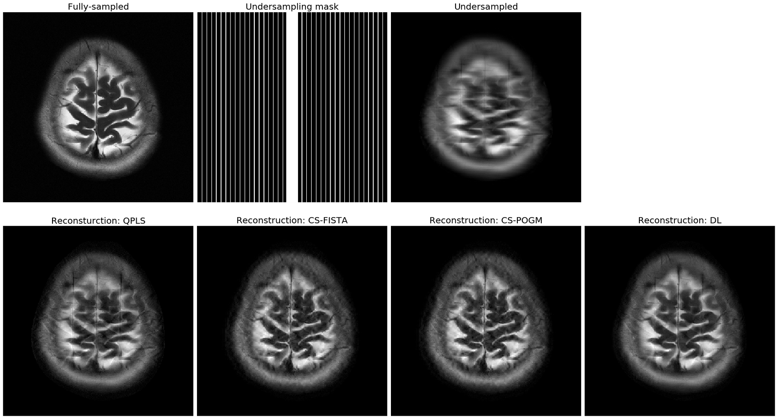
Figure 1. Reconstruction examples of Cartesian acquisitions. The sampling pattern here is an 7$$$\times$$$ 1D undersampling mask. QPLS stands for quadratic penalized least-squares, where the regularizer is a l2-norm of a finite-difference operator. We applied 40 CG iterations. CS stands for compressed sensing, where the regularizer is a l1-norm of a discrete wavelet transform (DWT). We applied 150 iterations for FISTA and 80 iterations for POGM. DL stands for dictionary learning [8].

Figure 2. Illustration of B0-informed reconstruction examples of non-Cartesian acquisitions. We used a dual-echo GRE sequence to estimate the B0 inhomogeneity map. For regularized reconstruction (QPLS, CS), we retrospectively subtracted 64 spokes from 320 spokes (5$$$\times$$$ undersampling.) QPLS means quadratic penalized least-squares. We applied 40 CG iterations. CS stands for compressed sensing, where the regularizer is a l1-norm of a discrete wavelet transform (DWT). We applied 80 iterations for POGM.
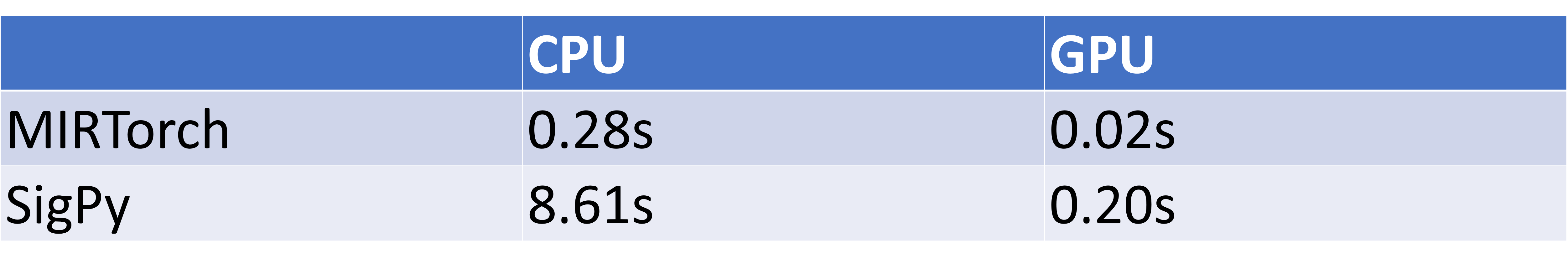
Table 1. Comparison of the proposed toolbox with Sigpy for computation time.
DOI: https://doi.org/10.58530/2022/4982