4972
Rapid Parameter Estimation for Combined Spin and Gradient Echo (SAGE) Imaging1Division of Neuroimaging Research, Barrow Neurological Institute, Phoenix, AZ, United States
Synopsis
In this study, we propose a generalized linear solution to estimate dynamic relaxation parameters R2* and R2 from combined spin- and gradient-echo (SAGE) MRI. We compared linear least squares (LLSQ) to nonlinear least squares (NLSQ) using Monte-Carlo simulated data and in vivo whole-brain data with varying signal-to-noise ratios (SNR). We show that using the LLSQ is both computationally more efficient and retains NLSQ precision, producing nearly the same estimates of R2* and R2 in a fraction of the time. This approach is widely extendable to other multi-echo, multi-contrast MRI methods, with applications including both perfusion MRI and functional MRI.
Introduction
Multi-echo, multi-contrast methods are increasingly used to quantify dynamic changes in transverse relaxation rates for applications in both dynamic susceptibility contrast (DSC)1,2 and functional MRI (fMRI).3,4 These methods produce hundreds of dynamic images with varying sensitivities to T1, T2*, and T2 effects across multiple echo times (TEs). The large amount of data generated from these scans creates a computational challenge to efficiently and accurately estimate voxel-wise relaxation parameters.Spin- and gradient-echo (SAGE) MRI relies on the acquisition of two gradient echoes (GRE), followed by two asymmetric spin echoes (ASE), and a spin echo (SE). Simplified SAGE, sSAGE, was proposed as an alternative approach with two GRE and one SE to avoid computationally expensive nonlinear fits at the expense of reduced echo data by leaving out ASEs.5,6 We propose a new analysis method that utilizes a linear least squares approach to obtain dynamic estimates of T2* and T2, with high computational efficiency, while retaining all echo readouts. We evaluated this using both simulated data and whole-brain data from a previously published DSC study.
Methods
The SAGE signal for a given TE can be modeled with a piecewise function according to:\[S(\tau) = \begin{cases}S_0^I e^{-\tau R_2^*} & 0 < \tau < \frac{TE_{SE}}{2} \\S_0^{II} e^{-TE_{SE}(R_2^*-R_2)-\tau(2 \cdot R_2 -R_2^* )} & \frac{TE_{SE}}{2} < \tau \leq TE_{SE}\end{cases}\]
where τ is each echo time, S0I and S0II are the signal intensity following the excitation and refocusing pulses, respectively, and which also include T1 effects, TESE is the spin echo TE, and R2* and R2 are the transverse relaxation rates (=1/T2* and 1/T2, respectively). This function can be solved using non-linear fitting7 or using an analytical solution 5,6, where the former is computationally expensive, and the latter uses a subset of echoes, i.e., not all acquired data.
Alternatively, we can represent equation 1 as a system of linear equations:
\[Ax=y\]
Matrix A comprises the constant coefficients, e.g, the echo times:
\[A=\begin{bmatrix}1 & 0 & -TE_1 & 0 \\1 & 0 & -TE_{GRE_n} & 0 \\\vdots & \vdots & \vdots & \vdots \\1 & -1 & -TE_{SE}+TE_{ASE_n} & TE_{SE}-2TE_{ASE_n} \\\vdots & \vdots & \vdots & \vdots \\1 & -1 & 0 & -TE_{SE} \\\end{bmatrix}\]
where TEGREn corresponds to the nth GRE TE, and TEASEn correspond to the nth ASE TE. The vectors x and y represent the variables and matrix constant products, e.g., fitting parameters and log transformed signal, respectively as:
\[x=\begin{bmatrix}ln(S_0^I) \\ln(\delta) \\R_2^* \\R_2\end{bmatrix}\]
\[y=\begin{bmatrix}ln(S_1) \\\vdots \\ln(S_n)\end{bmatrix}\]
Here Sn is the nth echo signal and δ =S0I/S0II. The pseudoinverse of A, i.e., A+, is then cross multiplied to the vector y.
To test this analysis method, we simulated two SAGE datasets by adding Rician noise with an SNR = 200 and another dataset with SNR = 20, each with 5 echoes, (TEs = 8.8, 26, 50, 68, 88 ms) R2* = 30 s-1, and R2 = 17 s-1. For in vivo analysis, we used SAGE-DSC images from a published dataset2 to assess efficiency and reliability compared to NLSQ fitting.
For simulated data, we compared the LLSQ and NLSQ estimation using probability density plots with average and standard deviations represented in Table 1. For in vivo data, we compared both methods at baseline (time point 1) and at the gadolinium (Gd) contrast peak, which represents an upper and lower signal-to-noise ratio, respectively. Lin’s concordance correlation coefficient (CCC) was used to assess agreement between the estimates for the in vivo data. Lastly, we compared the estimates with a probability density plot.
Results
Figure 1 shows R2* and R2 probability density function plots for the simulated data from nonlinear fitting and the linear solution, which shows nearly identical estimate curves for high SNR and low SNR. As seen in Table 1, the LLSQ and NLSQ solutions are very similar on average. Furthermore, at low signal to noise, the average values are nearly identical with the standard deviation becoming enlarged, as expected.Using in vivo whole-brain data, assessed in Figures 2, 3, and 4, we found that R2* and R2 estimates between the LLSQ and NLSQ solutions were nearly identical with most of the deviations in R2 for both baseline and max Gd, which was expected. Additionally, the fits are very similar as well with CCC > 0.990 between LLSQ and NLSQ for all estimates.
Lastly, the whole-brain non-linear fits required 48 minutes on a standard laptop CPU, while the linear solution can be achieved in just seconds on the same computer.
Discussion
In this study, we proposed a generalized linear least squares solution to estimate relaxation parameters from multi-echo and multi-contrast MRI methods, including SAGE but extendable to similar methods (GESFIDE8 and GESE-EPIK9). Our LLSQ method was verified in both simulated and whole-brain DSC data, with high agreement between nonlinear fit and analytical solutions for both R2* and R2. Importantly, large computational requirements are reduced through this linear solution.We anticipate that this method will enable rapid analysis of multi-echo, multi-contrast MRI data, including SAGE, for use in a wide range of applications. Limitations include possible nonuniform scaling in noisy log transformed data, however, at low SNR, the estimates were within acceptable tolerances.
Conclusion
We found that our method reduces computational time for estimating relaxation parameters from multi-echo, multi-contrast MRI, with high precision compared to nonlinear fits and while retaining all echo readouts.Acknowledgements
Barrow Neurological Foundation and Philips Healthcare.References
(1) Quarles, C. C.; Bell, L. C.; Stokes, A. M. Imaging Vascular and Hemodynamic Features of the Brain Using Dynamic Susceptibility Contrast and Dynamic Contrast Enhanced MRI. Neuroimage 2019, 187 (October 2017), 32–55. https://doi.org/10.1016/j.neuroimage.2018.04.069.
(2) Sisco, N. J.; Borazanci, A.; Dortch, R.; Stokes, A. M. Investigating the Relationship between Multi-Scale Perfusion and White Matter Microstructural Integrity in Patients with Relapsing-Remitting MS. Mult. Scler. J. - Exp. Transl. Clin. 2021, 7 (3), 205521732110370. https://doi.org/10.1177/20552173211037002.
(3) Keeling, E. G.; Bergamino, M.; Burke, A.; Steffes, L.; Stokes, A. M. Implementation of Multi-Contrast, Multi-Echo SAGE-FMRI in Aging and Alzheimer’s Disease. In Proceedings of the 29th Annual Meeting of ISMRM; 2021; p 1516.
(4) Bergamino, M.; Steffes, L.; Gonzales, A.; Karis, J. P.; Baxter, L. C.; Stokes, A. M. Optimization of Vascular and Functional Sensitivity Using Multi-Contrast, Multi-Echo SAGE-EPI for FMRI. In Proceedings of the 28th Annual Meeting of ISMR; 2020.
(5) Stokes, A. M.; Quarles, C. C. A Simplified Spin and Gradient Echo Approach for Brain Tumor Perfusion Imaging. Magn. Reson. Med. 2016, 75 (1), 356–362. https://doi.org/10.1002/mrm.25591.
(6) Stokes, A. M.; Skinner, J. T.; Yankeelov, T.; Quarles, C. C. Assessment of a Simplified Spin and Gradient Echo (SSAGE) Approach for Human Brain Tumor Perfusion Imaging. Magn. Reson. Imaging 2016, 34 (9), 1248–1255. https://doi.org/10.1016/j.mri.2016.07.004.
(7) Schmiedeskamp, H.; Straka, M.; Bammer, R. Compensation of Slice Profile Mismatch in Combined Spin- and Gradient-Echo Echo-Planar Imaging Pulse Sequences. Magn Reson Med 2012, 67 (2), 378–388. https://doi.org/10.1002/mrm.23012.
(8) Ma, J.; Wehrli, F. W. Method for Image-Based Measurement of the Reversible and Irreversible Contribution to the Transverse-Relaxation Rate. J. Magn. Reson. Ser. B 1996, 111 (1), 61–69. https://doi.org/10.1006/jmrb.1996.0060.
(9) Shah, N. J.; Silva, N. A.; Yun, S. D. Perfusion Weighted Imaging Using Combined Gradient/Spin Echo EPIK: Brain Tumour Applications in Hybrid MR‐PET. Hum. Brain Mapp. 2021, 42 (13), 4144–4154. https://doi.org/10.1002/hbm.24537.
Figures

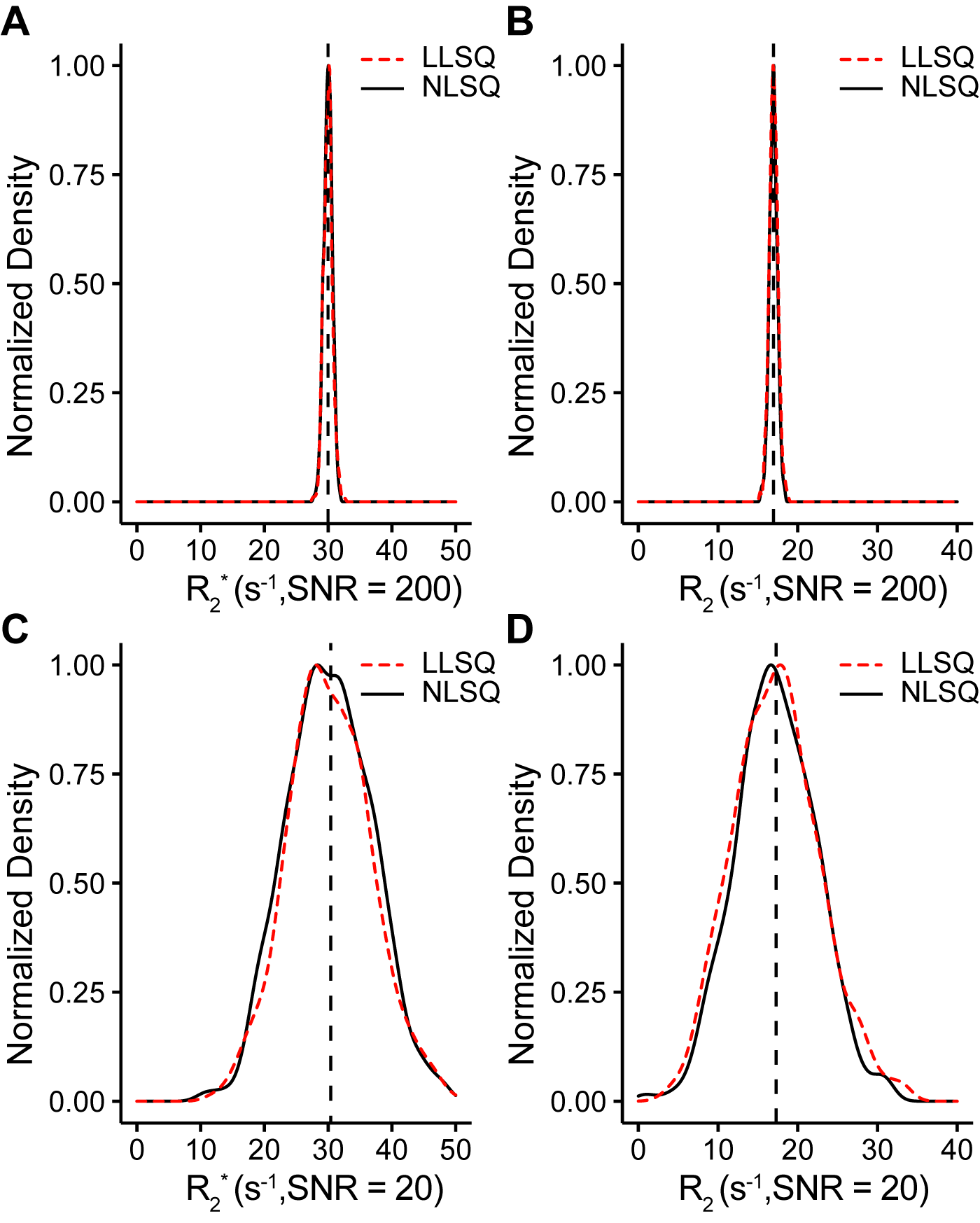
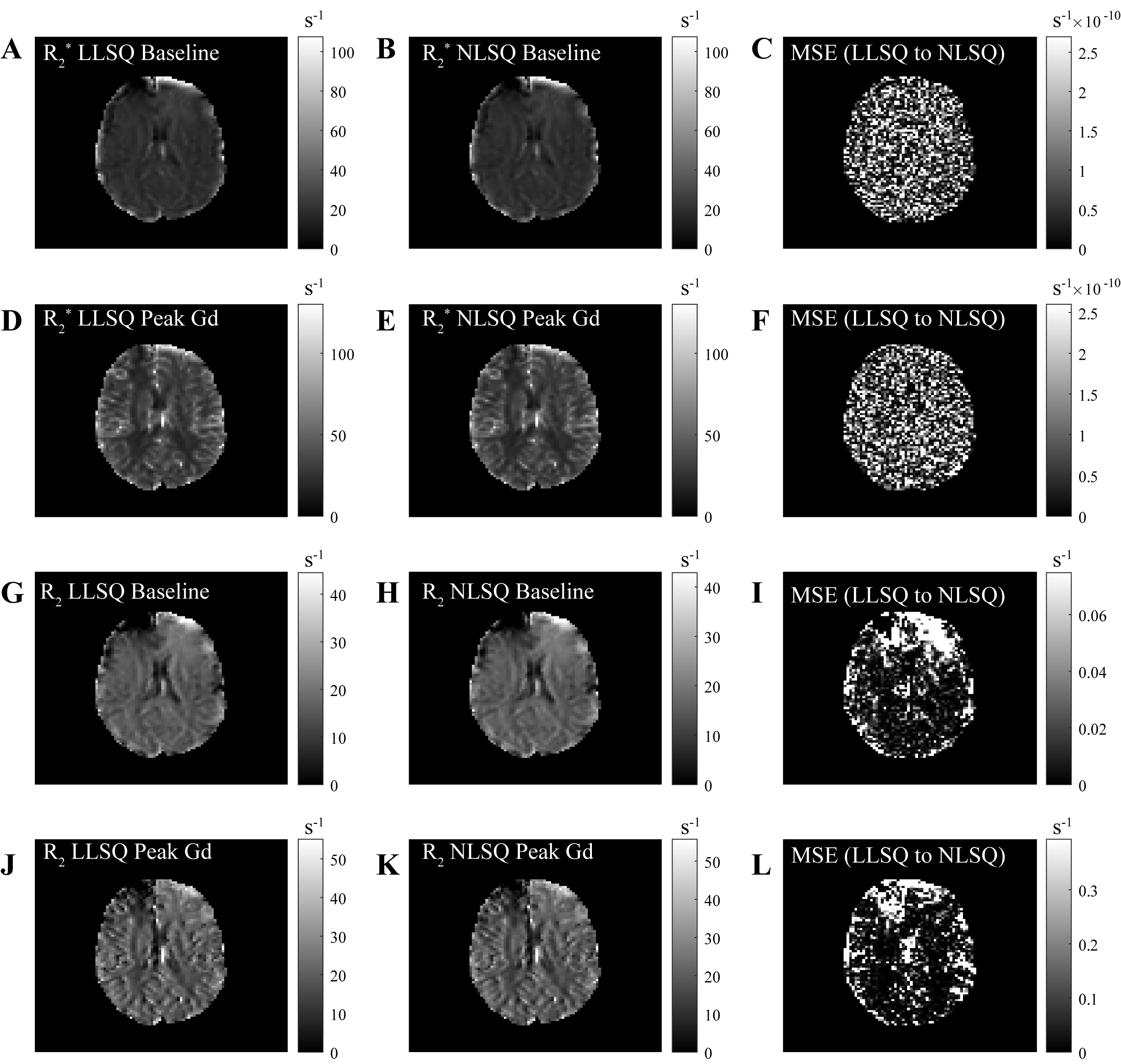
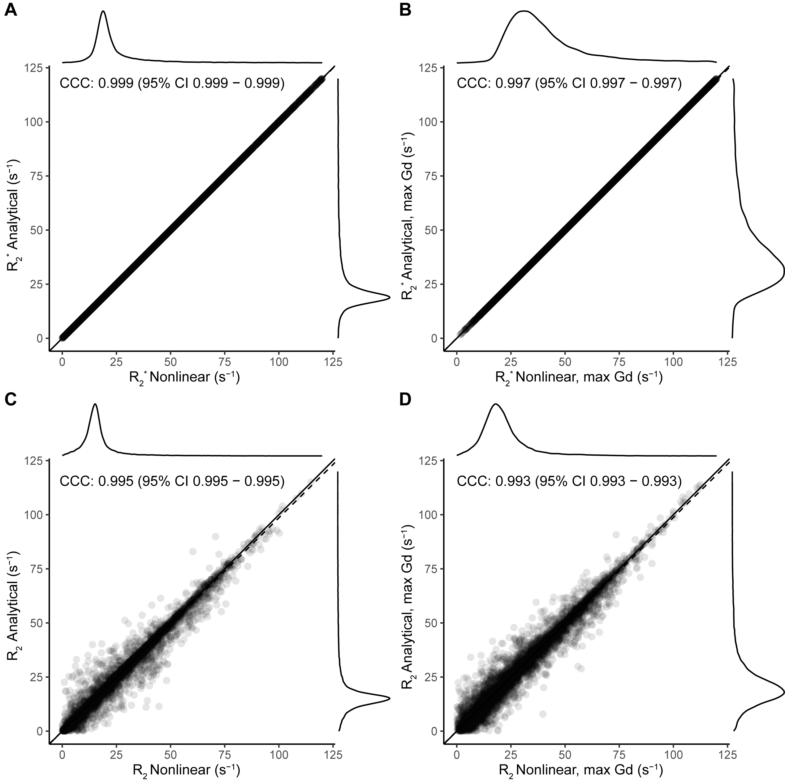
Figure 3 Comparison of the R2* and R2 from analytical and nonlinear solutions using the same slice as in Figure 2. Comparisons of R2* are shown in A and B for dynamic 1 and at maximum gadolinium bolus, respectively. Similarly, C and D show R2 for dynamic 1 and at maximum gadolinium bolus. Each of the plots show a high degree of agreement with CCC values approaching 1 for A and B and > 0.99 for C and D.
