4917
Venc Scouting with a Whole Volume Fourier Velocity Encoding Spectrum Acquisition1Radiology, Stanford University, Stanford, CA, United States, 2Radiology, Veterans Administration Health Care System, Palo Alto, CA, United States, 3Cardiovascular Institute, Stanford University, Stanford, CA, United States
Synopsis
We explored the application of acquiring Fourier Velocity Encoding (FVE) without spatial encoding to quickly estimate the velocity distribution within a volume of interest. One application is to allow for quick selection of Venc for a subsequent 4D-Flow acquisition, which can limit velocity aliasing and fine-tune the velocity-to-noise ratio for better data quality. Other applications may include new ways of looking at the pulsatility or turbulence of a volume of interest. In this work we implement a FVE sequence in Pulseq and run it in flow phantoms to demonstrate the proof-of-concept data of this technique.
Introduction
Phase contrast MRI allows for velocity of tissue to be recorded into the phase of the complex-valued data. Fourier velocity encoding (FVE) expands upon this idea by encoding with multiple velocity sensitivities, thereby allowing for intravoxel velocity distributions to be measured [1]. Several applications have been posed for this type of imaging [2,3], but FVE it is often limited by the long scan times to acquire many images with different velocity encodings.In this work, we explored the application of acquiring Fourier Velocity Encoding (FVE) without spatial encoding to quickly estimate the velocity distribution within a volume of interest. One application is to allow for quick selection of Venc for a subsequent 4D-Flow acquisition, which can limit velocity aliasing and fine-tune the velocity-to-noise ratio for better data quality. This has been demonstrated for 2D through plane flow [4], but not for the volumetric coverage and multidirectional encoding proposed here. Other applications may include new ways of looking at the pulsatility or turbulence of a volume of interest. In this work we implement a FVE sequence in Pulseq [5] and run it in flow phantoms to demonstrate the proof-of-concept data of this technique.
Methods
The FVE sequence used a non-selective excitation pulse with flip = 10°, followed by a bipolar gradient with duration = 6 ms, with variable gradient magnitude based on the targeted velocity encoding step (kv). The bipolar gradient was followed by a 1ms ADC segment and subsequent gradient spoiling simultaneously on all axes. The TE (time to beginning of FID) was 6.33 ms and TR = 9.54 ms. Fig 1 shows a portion of the pulse sequence used in this experiment.Velocity encoding was performed with 128 unique kv encodes with a velocity resolution of 5 cm/s, giving a velocity dynamic range of the measurement as [-320, 320] cm/s. To prevent steady state issues during pulsatile flow conditions, the kv ordering was randomized. 10000 total TRs were played for each directional encoding, requiring 1 minute of scanning per axes. Data was reconstructed by filtering the kv data with a Hamming window and then Fourier transforming to get a velocity spectrum.
The sequence was tested in a flow phantom loop with two different sized tubes (diameter = 16, 22 mm) going into (+Z) and out of (-Z) the scanner. Flow rates were controlled with a programmable flow pump (CardioFlow 5000 MR, Shelley Medical), with different constant flow rates (100, 150, 200 mL/s), as well as a pulsatile waveform. For pulsatile flow, the FVE data was retrospectively binned into 50ms temporal width bins to generate time resolved velocity spectra. Data was acquired on a Siemens 3T Skyra scanner.
The spectra were analyzed by comparing to a reference product 4D-Flow acquisition. First, the velocity spectrum was simulated from the 4D-Flow data for a qualitative reference. Second, the 4D-Flow peak velocities were calculated in the two flow tubes and reported as vmin (peak velocity in the -Z tube) and vmax (peak velocity in the +Z tube). The peak velocity was selected as the median of the top 5 velocities to remove outlier, high noise voxels at the edges of some vessels. vmin and vmax were also calculated from the FVE data by looking for the lowest velocity and highest velocity point that exceeded 3x the mean noise floor signal.
Results
Fig. 2A shows example 4D-Flow magnitude and velocity images from the flow phantom. Fig. 2B shows the velocity spectrum from the FVE data, and Fig. 2C shows the 4D-Flow derived spectrum. The maximum and minimum peak velocities estimated from the velocity spectra compared favorably (∆5 cm/s for vmin and ∆8.9 cm/s for vmax. Fig. 3A shows the acquired 4D-Flow data. Fig. 3B shows the different FVE velocity spectra for data acquired in the phantom with different flow rates. Fig 3C. compares the detected peak velocities between FVE and 4D-Flow for each flow rates. The mean absolute difference of these measurements was 5.9 ± 2.5 cm/s.Discussion
In this work we demonstrated acquisition of a full volume FVE velocity spectra using random kv ordering and retrospective binning in <3 minutes. Very good qualitative agreement was seen between the acquired FVE velocity spectrum and the spectra derived from 4D-Flow data. The detected peak velocities were on average 5.9 cm/s different between FVE and 4D-Flow, demonstrating accurate detection of the highest velocities and suitability for Venc selection. In all cases the FVE peak measurement was smaller than the 4D-Flow. When applied in a pulsatile phantom, the SNR was much lower due to binning the data into 20 different time frames, making peak detection in all time frames difficult, however velocity details are still evident. Future work will apply the methodology in human subjects and in more complicated flow distributions where the region of interest (e.g. stenotic jet) may be small. At this point the FVE sampling requirements (Kv steps, Kv range, and temporal bins) for different applications remain unclear. It may be necessary to selectively excite for the spatial excitation or change encoding schemes to maximize the data quality and acquisition efficiency.Acknowledgements
NIH Grant U01EB029427References
[1] Redpath, T. W., Norris, D. G., Jones, R. A., & Hutchison, J. M. (1984). A new method of NMR flow imaging. Physics in medicine and biology, 29(7), 891–895.
[2] Macgowan, C.K., Kellenberger, C.J., Detsky, J.S., Roman, K. and Yoo, S.-J. (2005), Real-time Fourier velocity encoding: An in vivo evaluation. J. Magn. Reson. Imaging, 21: 297-304.
[3] Hansen, Michael S., et al. "Accelerated dynamic Fourier velocity encoding by exploiting velocity-spatio-temporal correlations." Magnetic Resonance Materials in Physics, Biology and Medicine 17.2 (2004): 86-94.
[4] Galea, Daniela, M. Louis Lauzon, and Maria Drangova. "Peak velocity determination using fast Fourier velocity encoding with minimal spatial encoding." Medical Physics 29.8 (2002): 1719-1728.
[5] Layton, K.J., Kroboth, S., Jia, F., Littin, S., Yu, H., Leupold, J., Nielsen, J.-F., Stöcker, T. and Zaitsev, M. (2017), Pulseq: A rapid and hardware-independent pulse sequence prototyping framework. Magn. Reson. Med., 77: 1544-1552.
Figures
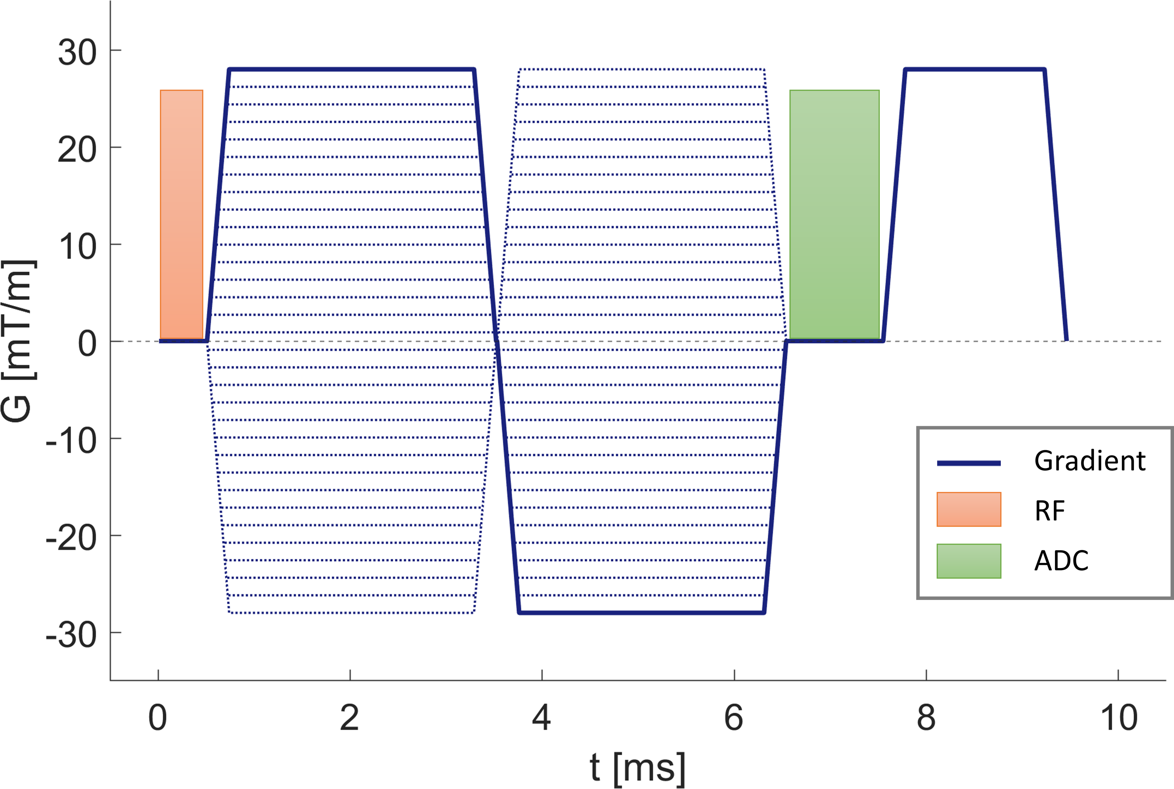
Figure 1: A depiction of a single TR of the FVE pulse sequence. Dotted lines show the different kv encodes (32 kv encodes are depicted compared to actual acquired kv=128).

Figure 2: A) Axial and coronal views of the flow phantom used in the study, with both magnitude and velocity data depicted. B) measured FVE velocity spectrum of the data, normalized so the maximum value = 1, and cropped on the y-axis owing to the high the static tissue signal (v = 0). C) The 4D-Flow derived spectrum of the same flow conditions. B) and C) both show dotted red lines depicting their respective measurements of vmin and vmax.

Figure 3: A) Shows coronal velocity images of the flow phantom with the same velocity range for three different flow rates. B) Shows the velocity spectra measured for each of the different flow rates. C) Shows the measured vmin and vmax from the FVE data and the 4D-Flow data, for each flow rate.

Figure 4: FVE velocity spectrum in the phantom with a pulsatile flow waveform, showing 4 of the 20 timeframes, including the peak flow timeframe (top right).