4887

MR measures of regional cerebral blood flow and cortical thickness are tightly linked to the proximity of large cerebral arteries

Samantha Cote¹, Marco Perez Caceres¹, Felix Dumais¹, Jean-Francois Lepage¹, and Kevin Whittingstall¹
¹Université de Sherbrooke, Sherbrooke, QC, Canada

Synopsis

Using time of flight magnetic resonance angiography, we explored how local variations in cerebral arterial morphology are related to cerebral blood flow (CBF) and cortical thickness (CT). We observed a significant, negative relationship between the proximity of a region of interest to an artery and CBF and CT such that regions proximal to large arteries have higher CBF and CT. These results highlight the importance of considering underlying cerebral vasculature when studying the human brain using MRI as it can lead to significant biases in commonly employed metrics.

Introduction

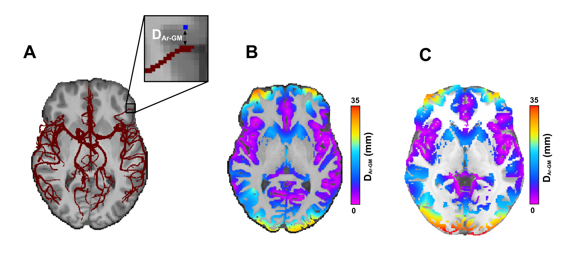
Structural and Hemodynamic brain markers derived from magnetic resonance imaging (MRI) are common, non-invasive methods used to study brain function and structure in humans^1,2. While these methods have aided in the advancement of our understanding of the human brain in both healthy and pathological states, there is emerging evidence that local cerebral vascular structure may have an impact on estimates cerebral blood flow (CBF)^3–5 and cortical gray matter thickness (CT)⁶. However, the effect of the proximity of large cerebral arteries on estimates of CBF and CT has yet to be examined.
Time of Flight (TOF) magnetic resonance angiography is an excellent method to visualize cerebral arteries from which image segmentation methods can be used to quantify the cerebral vascular tree^7,8. However, using the segmented maps in conjunction with other modalities like arterial spin labeling (ASL) and T1-weighted imaging remains difficult. First, traditional registration methods distort arterial trees when warping to standard space⁷. Second, distal regions of the arteries are lost when averaging across participants due to high intrasubject variability⁷. Therefore, we propose a method to address these limitations by extracting the distance between a voxel of interest and its nearest arterial voxel in native space and assigning the distance value to the voxel of interest. This is repeated for every voxel in the brain creating a whole-brain map of local vascular information. This vascular map can be transformed into standard space, segmented into tissue classes of interest, and averaged across participants without distorting the information and compared with other MRI modalities. In the present study, we apply this method to investigate the effect of the proximity of large cerebral arteries on estimates of CBF and CT.

Methods

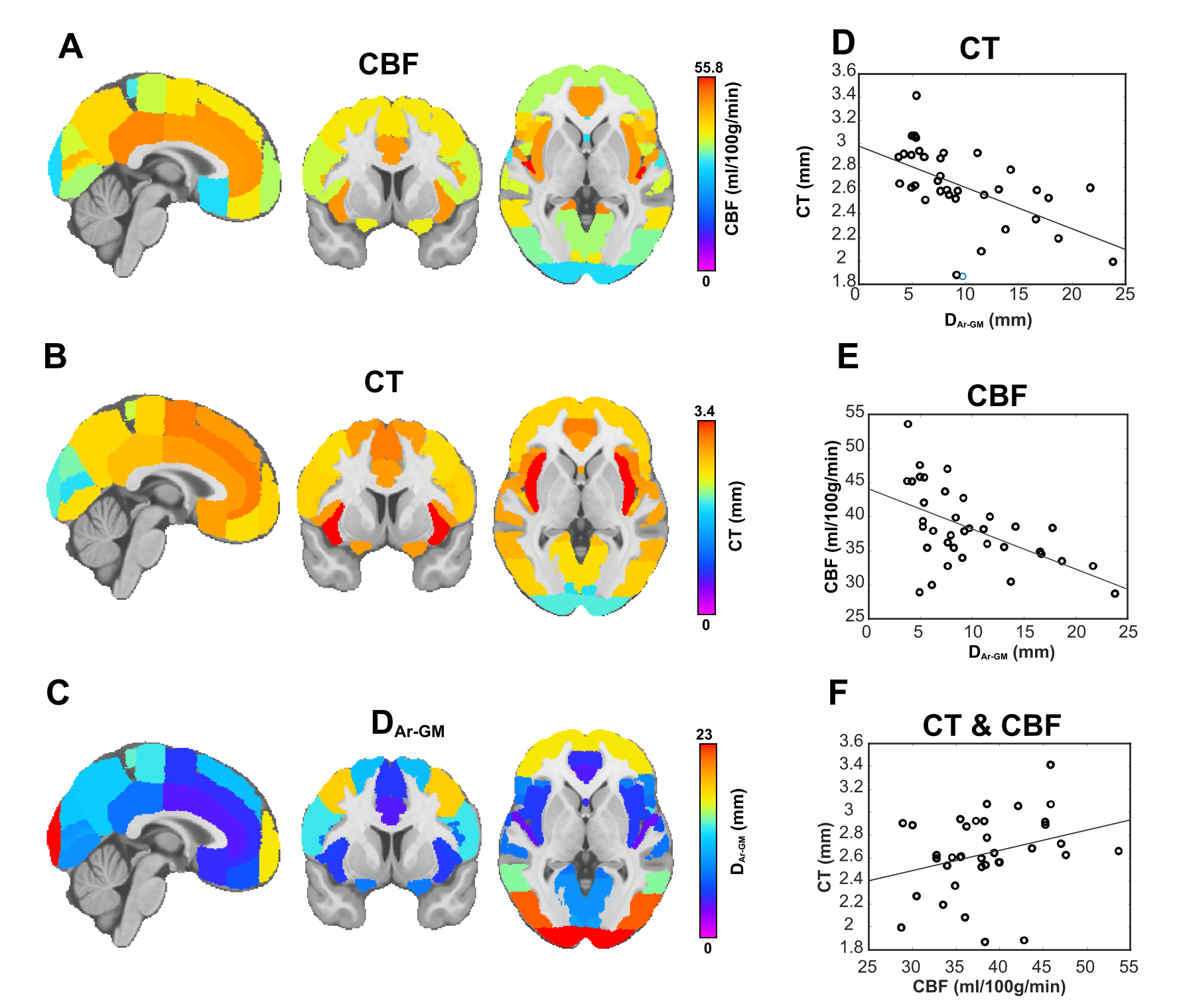
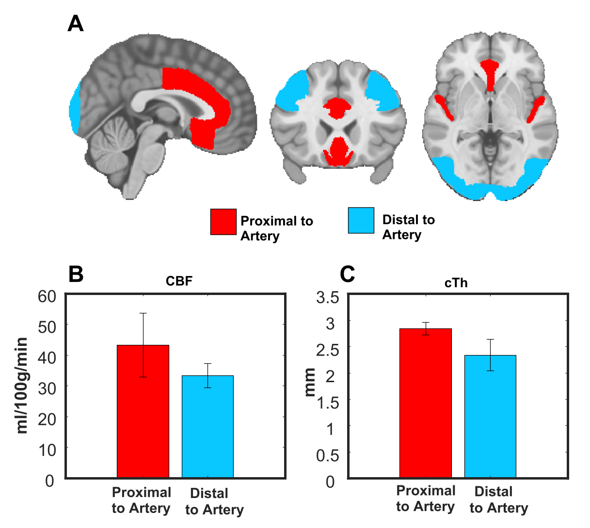
Thirteen participants were imaged on a 3T Ingenia scanner equipped with a 32-channel head-coil (Philips Healthcare, Best, Netherlands). First, a 3D gradient-echo T1 weighted image was collected (field of view (FOV)=240X240X161 mm; TR/TE=7.9/3.5ms, 1 mm isotropic voxels, flip angle(FA)= 8°), followed by a high resolution, whole-brain multi-band TOF image (FOV= 200X200X120.9mm, TR/TE= 23/3.45ms, FA= 18°, parallel imaging (SENSE) acceleration factor=3, acquisition resolution of 0.65X0.65X1.30, reconstructed resolution of 0.626x0.625x0.65mm) and lastly pseudo-continuous ASL (pCASL) sequence (background suppression, label duration=1650ms, postlabel delay (PLD)=1800ms, 2D multislice EPI readout, TR/TE 4246/16ms, 22 4mm slices, 3x3 resolution, FOV=240X240mm) was acquired. Each participant’s TOF image was registered using a rigid transformation to the participant’s T1 image. The cerebrovascular arteries were segmented using vessel enhancement diffusion followed by strict hysteresis thresholding base on the parameters of a gaussian mixture model clustering. Hypothetic false positive values were removed using a watershed algorithm by only keeping segmented vascular voxels that were linked to the Circle of Willis^7,8. Next, the binary, denoised segmentations were visually inspected and veins were removed. The vascular tree was then skeletonized and the distance between each voxel and its closest arterial voxel was computed (D_Ar-GM; see Figure 1 for visual representation) using the Scikit-image and Scipy python packages^9,10. Next, the D_Ar-GM map was warped to the MNI 152 asymmetric brain template^11,12 for group analysis. pCASL images were processed using ExploreASL¹³. Cortical thickness (CT) was extracted using FreeSurfer¹⁴ and warped to MNI 152. Next, gray matter (GM) CBF and CT were correlated with D_Ar-GM across 36 ROIs from the Harvard-Oxford Atlas¹⁵ using the Spearman rank correlation. Lastly, CBF and CT were compared in the regions where D_Ar-GM was above the 90th percentile (regions distal to arteries; D_Ar-GM above 20.47 mm) and below the 10th percentile (regions proximal to arteries; D_Ar-GM below 4.16 mm).

Results

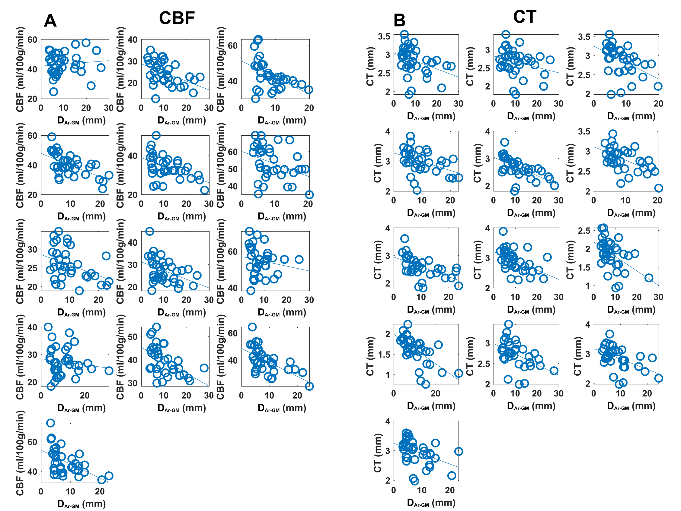
The average D_Ar-GM, CBF, CT in each ROI are shown in Figure 2A-C. CBF (ρ=-0.55, p<0.01) and CT (ρ=-0.64, p<0.01) were negatively correlated with D_Ar-GM (Figure 2D-E), this relationship was strongest between CT and D_Ar-GM and present in all participants (Figure 3). CBF and CT had a positive relationship (ρ=0.35, p=-.03; Figure 2F). CBF and CT were significantly higher in regions proximal to an artery (Figure 4), compared to regions distal to an artery (CBF: t=-6.71, p<0.0001; CT: t=-14.12, p<0.0001).

Discussion

We investigated the effect of large cerebral arteries on CBF and CT and observed a strong, negative relationship between D_Ar-GM and local CBF and CT. Specifically, the closer a region is to a large artery the higher the estimate of CBF and CT are. The negative relationship between D_Ar-GM and CT might be due to the T1-signal in arteries near the GM influencing the T1-signal of the GM. This would lead to a bias in the contrast of the GM leading to the appearance of more gray voxels resulting in a larger estimate of CT. The relationship between large arteries and CBF is likely due to higher bolus concentrations within the branches of the cerebral arteries biasing local GM estimates of CBF. Our results give further support that local arterial morphology is an important biomarker to consider when studying the brain. Failure to do so may lead to important bias in the neurophysiological interpretation of the MRI results. This may be especially important when studying clinical groups where the integrity of the cerebrovascular system may be affected.

Acknowledgements

We would like to thank our participants for their time, and Felix Janelle and Maxime Chagnon for their feedback.

References

1. Lerch JP, van der Kouwe AJW, Raznahan A, et al. Studying neuroanatomy using MRI. Nature Neuroscience. 2017;20(3):314-326. doi:10.1038/nn.4501

2. Clement P, Mutsaerts HJ, Václavů L, et al. Variability of physiological brain perfusion in healthy subjects-A systematic review of modifiers. Considerations for multi-center ASL studies. Journal of Cerebral Blood Flow & Metabolism. 2018;38(9):1418-1437. doi:10.1177/0271678X17702156

3. Chen Y, Wang DJJ, Detre JA. Comparison of arterial transit times estimated using arterial spin labeling. Magnetic Resonance Materials in Physics, Biology and Medicine. 2012;25(2):135-144. doi:10.1007/s10334-011-0276-5

4. Hu Y, Lv F, Li Q, Liu R. Effect of post-labeling delay on regional cerebral blood flow in arterial spin-labeling MR imaging. Medicine. 2020;99(27):e20463. doi:10.1097/MD.0000000000020463

5. Alsop DC, Detre JA, Golay X, et al. Recommended implementation of arterial spin-labeled Perfusion mri for clinical applications: A consensus of the ISMRM Perfusion Study group and the European consortium for ASL in dementia. Magnetic Resonance in Medicine. 2015;73(1):102-116. doi:10.1002/mrm.25197

6. Tardif CL, Steele CJ, Lampe L, et al. Investigation of the confounding effects of vasculature and metabolism on computational anatomy studies. NeuroImage. 2017;149(September 2016):233-243. doi:10.1016/j.neuroimage.2017.01.025

7. Bernier M, Cunnane SC, Whittingstall K. The morphology of the human cerebrovascular system. Human Brain Mapping. 2018;(July):1-14. doi:10.1002/hbm.24337

8. Bizeau A, Gilbert G, Bernier M, et al. Stimulus-evoked changes in cerebral vessel diameter: A study in healthy humans. Journal of Cerebral Blood Flow and Metabolism. 2018;38(3):528-539. doi:10.1177/0271678X17701948

9. Pedregosa FABIANPEDREGOSA F, Michel V, Grisel OLIVIERGRISEL O, et al. Scikit-Learn: Machine Learning in Python Gaël Varoquaux Bertrand Thirion Vincent Dubourg Alexandre Passos PEDREGOSA, VAROQUAUX, GRAMFORT ET AL. Matthieu Perrot. Vol 12.; 2011. http://scikit-learn.sourceforge.net.

10. Virtanen P, Gommers R, Oliphant TE, et al. SciPy 1.0: fundamental algorithms for scientific computing in Python. Nature Methods. 2020;17(3):261-272. doi:10.1038/s41592-019-0686-2

11. Fonov V, Evans AC, Botteron K, Almli CR, McKinstry RC, Collins DL. Unbiased average age-appropriate atlases for pediatric studies. NeuroImage. 2011;54(1):313-327. doi:10.1016/J.NEUROIMAGE.2010.07.033

12. Fonov V, Evans A, McKinstry R, Almli C, Collins D. Unbiased nonlinear average age-appropriate brain templates from birth to adulthood. NeuroImage. 2009;47:S102. doi:10.1016/S1053-8119(09)70884-5

13. Mutsaerts HJMM, Petr J, Groot P, et al. ExploreASL: An image processing pipeline for multi-center ASL perfusion MRI studies. NeuroImage. 2020;219(June). doi:10.1016/j.neuroimage.2020.117031

14. Fischl B, Dale AM, Raichle ME. Measuring the Thickness of the Human Cerebral Cortex from Magnetic Resonance Images. www.pnas.org

15. Desikan RS, Ségonne F, Fischl B, et al. An automated labeling system for subdividing the human cerebral cortex on MRI scans into gyral based regions of interest. NeuroImage. 2006;31(3):968-980. doi:10.1016/J.NEUROIMAGE.2006.01.021

Figures

Figure 1. An arterial segmentation (A; shown in red) over T1- image in native space to demonstrate how D_Ar-GM is computed. The inset in (A) illustrates how the shortest distance is calculated from a GM voxel to the closest arterial voxel, this distance is then assigned to the GM voxel. This is repeated for all GM voxels to generate a map of D_Ar-GMthroughout the brain (an example of a D_Ar-GM map in one participant is shown in B). The D_Ar-GM map is then warped to MNI to be used for group analysis (example in one participant shown in C) and regional variations in vascular information is maintained.

Figure 2. Average CBF, CT and D_Ar-GM in the ROIs of the Harvard Oxford Atlas. CBF and CT are significantly, negatively correlated with D_Ar-GM (p<0.01). CBF and CT are positively correlated (p<0.05). Each point represents an ROI.

Figure 3. Individual scatter between CBF, CT and D_Ar-GM across ROIs in each participant. The relationship was stronger and more consistent for CT, the average correlation coefficient was -0.48 and significant in 12 of 15 participants while the average correlation coefficient for CBF was -0.38 and significant in 10 of 15.

Figure 4. CBF and CT are significantly higher in the regions proximal to an artery (D_Ar-GM below 4.16 mm) compared to regions distal to an artery (D_Ar-GM above 20.47 mm; CBF: t=-6.71, p<0.01; CT: t=-14.12, p<0.01).

Proc. Intl. Soc. Mag. Reson. Med. 30 (2022)

4887

DOI: https://doi.org/10.58530/2022/4887