Introduction

Dynamic MRI is a promising tool to visualize articulatory changes in both functional and structural scales, providing unprecedented opportunities for linguistic studies. Recent methods have enabled drastic improvements in imaging speed and spatial coverage.^1,2 Both high spatial and temporal resolutions are needed for speech MRI because of the short time of articulatory changes and fine details of muscle movements.
In the current work, we expand the previous methods to high (near) isotropic resolution (1.875 mm) with significant coverage of 32 3D 2-mm slices and an overall 3D volume acquisition rate of 35 Hz.¹ By applying this method and analyzing concurrently recorded and synchronized audio waveforms, we are able to observe complex movements during speech, such as lateral tongue deformation during the American English voiced lateral [l] as compared to (central) [t]. To our knowledge, our work represents the highest coverage and highest resolution 3D dynamic images of speech to date.

Methods

We implemented a low rank constraint and spatial regularized partial separability (PS) model for the dynamic speech images.^1,2,3,4 The PS model leverages strong spatiotemporal correlations in the dynamic images during speech and represents the time series of volumes as a combination of temporal and spatial basis functions, a low rank expansion of the image series.¹ 3D imaging requires significant time to fully sample the low rank model, especially as the number of kz locations increases to provide more isotropic voxels. We acquired a 3D sagittal acquisition with a 128-matrix size with a 24 cm field of view and 32 kz-slices with 64 mm full thickness, for a spatial resolution of 1.875×1.875× 2mm. We also provide a temporal resolution of 35 fps with 4 imaging lines acquired per navigator. We perform 40 full-frame measurements for which the total duration of the scan is less than 20 minutes resulting in 40960 reconstructed images from the PS model at 35 frames per second. This data was acquired while volunteer subjects read the ‘Rainbow Passage’ nine times during the 20-minute scan.

Results

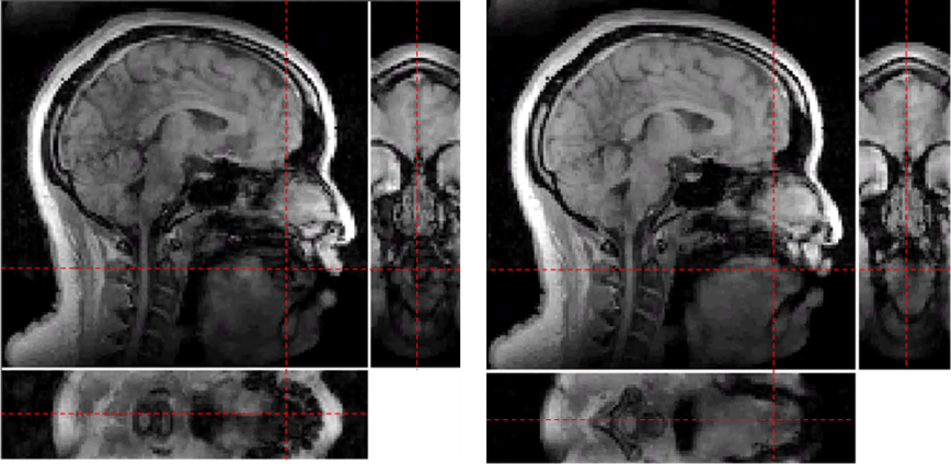
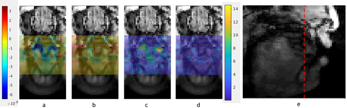
To visualize the capability of this method to differentiate articulatory movements in 3 dimensions, we choose to compare the tongue position in the (lateral) [l] and (central) [t] of the American English words ‘look’ and ‘token’. The lingual characteristics of these alveolar consonants differ minimally in a way uniquely suited to observation using 3D imaging. While the consonants share the same place of articulation, air flows over the side(s) of the tongue during [l] but not during [t]. Studying the unique geometry of [l] requires us to visualize the coronal and sagittal planes of the tongue simultaneously; the axial plane can help confirm observations made in the other two. Figure 1 illustrates a single frame of the 3D data in all three planes. This allows us to capture the unique twisting deformation of the tongue during [l]; as predicted, the tongue is not deformed in this way during [t].
To demonstrate that we are able to reliably measure the significant difference between the tongue posture in [l] and [t], we present another sample, [l] in the word ‘light’. Figure 2 shows the magnitude subtraction map and t-test map of [l]ook, [t]oken, and [l]ight matched with anatomical coronal images. The t-test was performed across the 9 repetitions during the full speech sample. The value shown for the t-test map is $$$i=-log⁡(p_i)$$$ where $$$p_i$$$ are the t-test p-values of each voxel. The larger difference in (a) than (b) and higher signal in (c) than (d) illustrate the difference of signal intensity between [l] and [t] is much bigger than between the two different [l]’s. We note, for example, how successfully our method captures the predicted difference in how the lowered sides of the tongue contribute to the unique geometry of [l] versus [t].
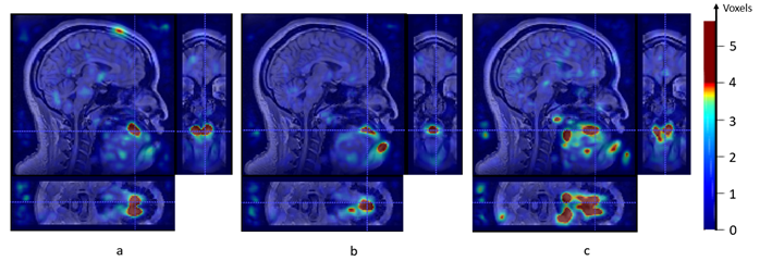
Another demonstration is the deformation magnitude maps of three speech samples. We calculate the deformation map from resting state to sample states. The value in the maps indicates the approximate number of voxels that move from resting state to sample states. In figure 3, (a) and (b) show the main moving structure of sample [l] is the tongue tip while [t] shows remarkably clear evidence of coarticulation with both the upcoming velar [k] and nasal [n] of ‘token’.

Discussion

This method allows us to make unique and highly detailed observations about the static geometry of complex gestures like the tongue grooving and twisting associated with [l]. It also allows us to make fine-grained and compelling observations about the nature of coarticulation. For example, we present evidence of simultaneous anticipatory velic lowering, velum raising, and lip rounding all during the ‘simple’ alveolar stop [t] of ‘token’. In future work we will examine ways to better visualize articulatory differences in this high dimensionality data in order to address issues of linguistic relevance.

Conclusion

By applying sparse sampling navigators and PS model, we managed to increase the 3D coverage of dynamic speech magnetic resonance imaging to 32 slices with 64 mm full thickness with near-isotropic spatial resolution of 1.875×1.875× 2mm and temporal resolution of 35 fps. This shows great potential in capturing small but highly consequential articulatory differences in speech samples from natural speech while reading passages.

Acknowledgements

Research reported in this publication was supported by the National Institute Of Dental & Craniofacial Research of the National Institutes of Health under Award Number R01DE027989. The content is solely the responsibility of the authors and does not necessarily represent the official views of the National Institutes of Health.