4823
Workflow for Personalized RF Safety Assessment of Orthopedic Implants in MRI, a Proof of Concept1Computational Imaging, UMC Utrecht, Utrecht, Netherlands, 2Biomedical Engineering, Eindhoven University of Technology, Eindhoven, Netherlands, 3Radiology, UMC Utrecht, Utrecht, Netherlands, 4Eindhoven University of Technology, Eindhoven, Netherlands
Synopsis
Patients with non-labelled implants are often ineligible for MRI. Sometimes non-labelled implants are scanned by some hospitals based on literature and empirical insights, power constraints are abided to avoid tissue heating. Using an accelerated simulation method we demonstrate a proof of concept workflow to obtain the patient-specific SAR increase for multiple patient and implant positions within 2-3 hours. This workflow uses two orthogonal X-ray images to construct a 3D model of the implant which is inserted in a human model. The method enables more accurate scanning constraints and, a more informed risk vs benefit analysis for each patient.
Introduction
Magnetic resonance imaging (MRI) is a very safe imaging modality, however, for patients with medical implants there are risks associated with undergoing an MRI examination. One risk is that the implant can couple with the radiofrequency (RF) transmit coil causing a high specific absorption rate (SAR) around the implant. To mitigate this the average power over the time of the scan delivered by the RF transmit coil is limited resulting in longer scan times or poorer image quality. For non-labelled non-ferromagnetic implants, there is no indication of the extent of the increase of the SAR around the implant. As a result, those patients are not scanned at all, or for some implants in some hospitals, these patients are scanned with overly conservative scanning restrictions based on literature and physical insights. It would be ideal to have a patient-specific indication of the potential heating, enabling scanning of these patients in more hospitals using a more accurate assessment of scanning restrictions.Determining patient-specific RF heating is a computationally demanding task. Simulating a single configuration of patient, implant, and RF coil can take several hours1,2. Therefore, it is currently unfeasible to simulate multiple configurations for an indication of the RF heating.
Previously, we have presented the update method that greatly reduces the simulation time3. The implant is considered a small perturbation of the simulated configuration, and given the incident RF fields when the implant is not present, the scattered RF fields resulting from the implant can be calculated within seconds or minutes.
In this work, we use the update method to demonstrate a workflow to predict the patient-specific RF heating. Ideally, this workflow should be quick (< 45min), fully automated where only a review of intermediate steps is required, and a final version should be able to be performed by a technician.
Methods
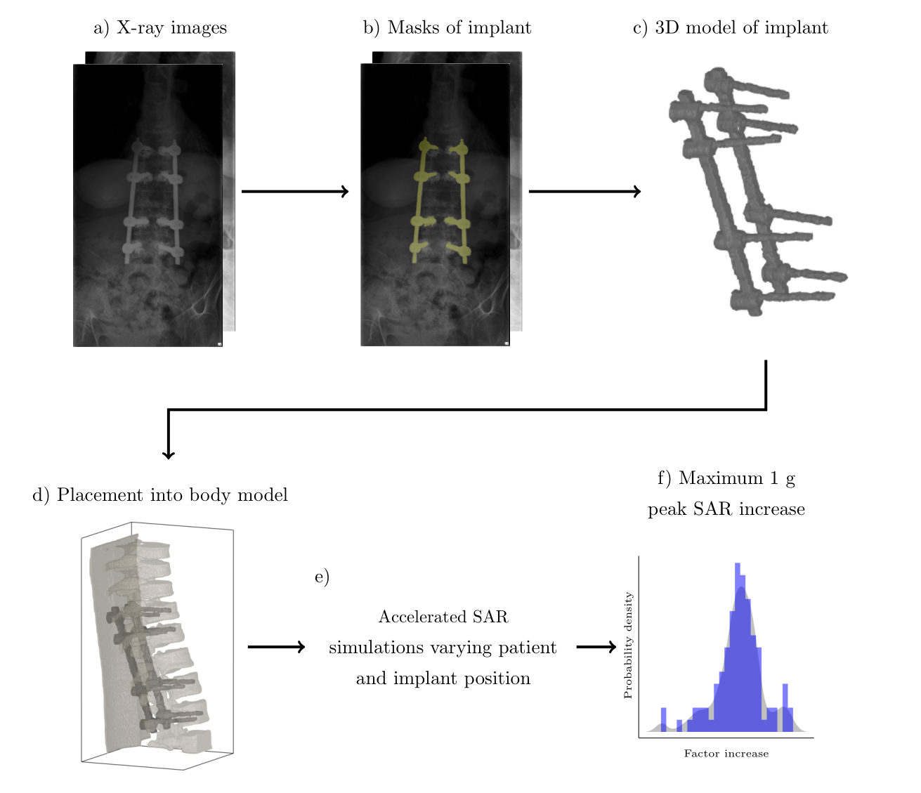
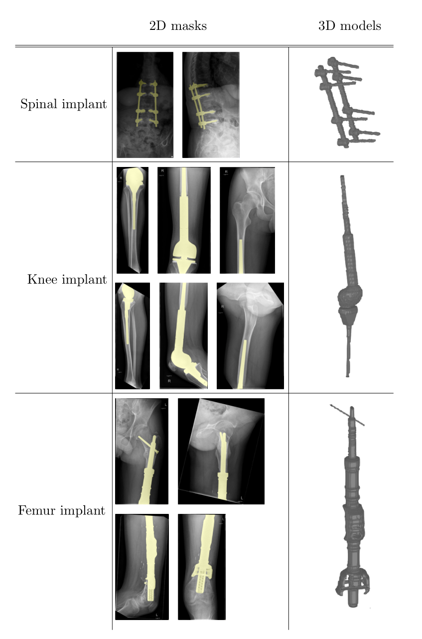
The proposed workflow overview is shown in Figure 1. The first step of the workflow is to obtain the location and geometry of the implant by using two orthogonal X-ray images (often already available), in which the implant is segmented obtaining 2D masks. Using trivial a priori information about the implant geometry or even knowing the type of implant, a 3D model can be constructed. This model is then placed inside a virtual family member that resembles the patient most (i.e. Duke in our case). Afterward, the update method is used to obtain the SAR increase around the implant for various patient and implant positions.The proposed workflow is demonstrated on three patients with various implants, shown in Figure 2. The 3D models are constructed using simple in-house developed tools.
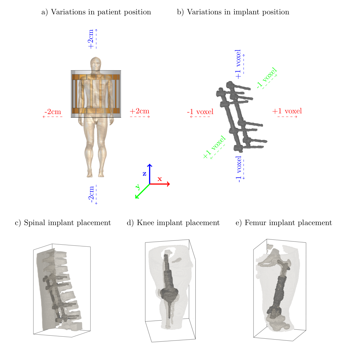
To more accurately predict the SAR increase with potential uncertainties in patient and implant position, we simulate 5 patient positions and 27 implants positions, Figure 3. After removing unrealistic configurations with implants protruding from skin or bone, we were left with 105, 90, and 65 simulations for the spinal, knee, and femur implant, respectively.
Results and Discussion
Segmenting the implant in the X-ray images took less than 5 mins for all images. Creating the 3D model was done in 5-10mins per implant. Finally, the placement within the human model took another 10 mins per implant. All combined, the total setup time for the simulations takes around 15-20 mins per implant. However, these tasks can be further automated to accelerate this procedure, for example, by using an automatic segmentation approach, and by creating templates for different implant types and placements within the human body model.The simulations were done in 166, 135, and 97.5mins for the spinal, knee, and femur implant respectively, between 58 and 234 times faster than FDTD simulations.
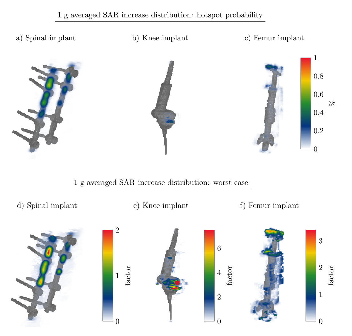
From the simulations we extract the 1g averaged SAR around the implant. Using this information we can create a heatmap that indicates where the SAR hotspot around the implant will most likely occur (Figure 4a-c). This likelihood is defined as$$P_{SAR}(\vec{r}) = \frac{1}{N}\sum_{i = 1}^{N} \frac{SAR_i(\vec{r})}{max(SAR_i(\vec{r}))}$$With$$$\,N\,$$$ as the number of simulations, and$$$\,SAR_i(\vec{r})\,$$$ the SAR distribution for a single simulation. We observe, for example, that for the knee implant the SAR hotspot will occur in the fluid around the joint.
Furthermore, the worst-case scenarios are shown in Figure 4d-f. The stated factor is the 1g averaged SAR increase with respect to the 1g averaged peak SAR in the calculated volume when the implant is not present. This factor can also be calculated with respect to the actual peak value of the entire body when the implant is not present.
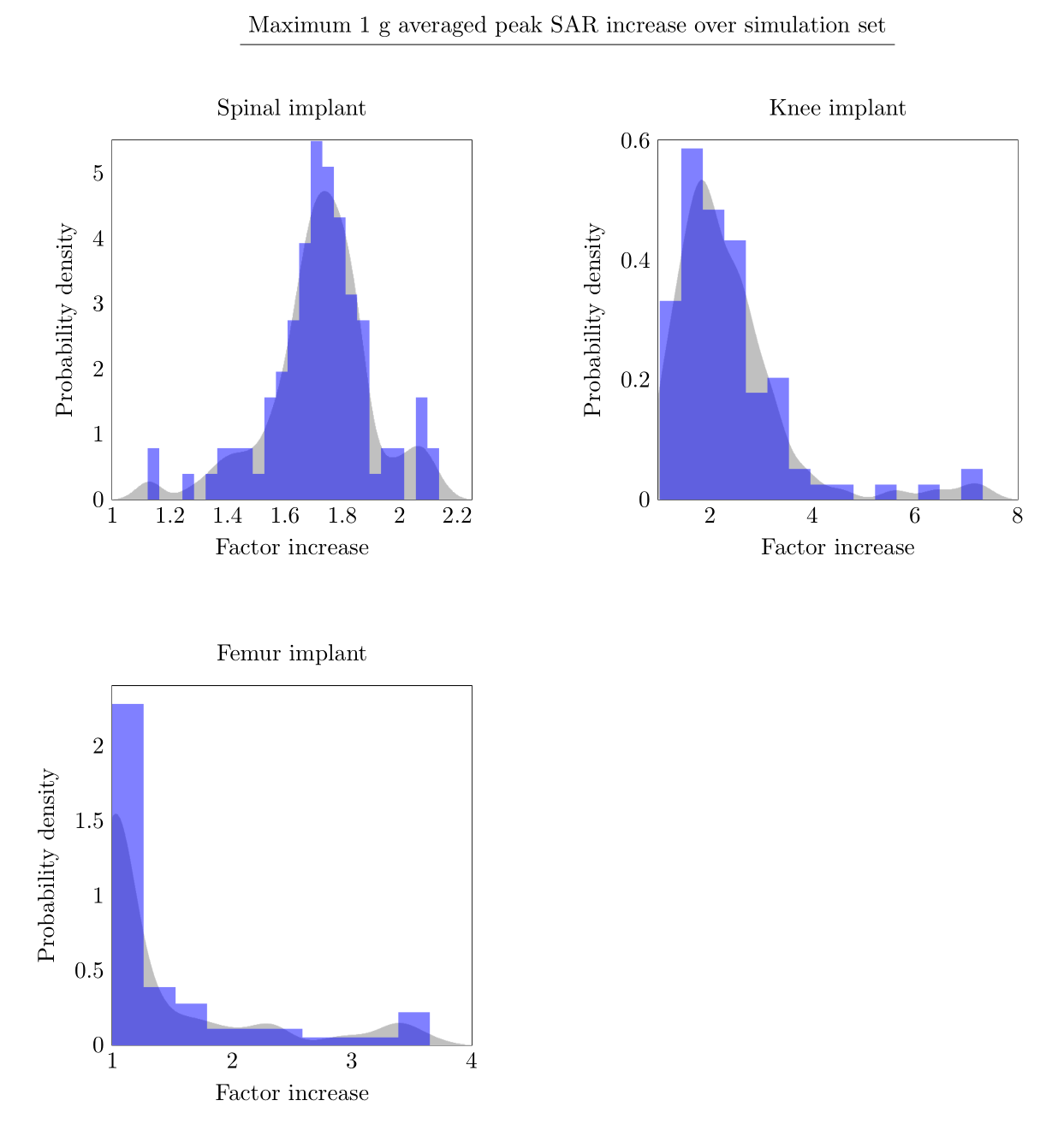
Based on all the simulations for an implant, we can determine the distribution of the peak 1g averaged SAR increase. This is shown in Figure 5. From this distribution, a more informed decision can be made about scanning constraints and the patient-specific risk vs benefit.
Eventually, when this workflow is further automated it can be used in the clinic to scan patients with non-labelled implants, or potentially alleviate scanning restrictions for labelled implants. This workflow can be performed in the days before the patient comes in for an MRI examination.
Conclusion
We demonstrate a proof of concept workflow to determine the patient-specific RF heating around implants. Using this methodology, patients with non-labelled implants can potentially be scanned.Acknowledgements
No acknowledgement found.References
1. Guerin, B. et al. Realistic modeling of deep brain stimulation implants for electromagnetic MRI safety studies. Physics in Medicine & Biology 63 (2018).
2. Cabot, E. et al. Evaluation of the rf heating of a generic deep brain stimulator exposed in 1.5 T magnetic resonance scanners. Bioelectromagnetics 34, 104–113 (2013).
3. Stijnman, P. R. S. et al. Accelerating implant RF safety assessment using a low-rank inverse update method. Magnetic Resonance in Medicine 83, 1796–1809 (2020).
Figures