4811

Improving the accessibility of deep learning-based denoising for MRI using transfer learning and self-supervised learning

Qiyuan Tian¹, Ziyu Li², Wei-Ching Lo³, Berkin Bilgic¹, Jonathan R. Polimeni¹, and Susie Y. Huang¹
¹Martinos Center for Biomedical Imaging, Massachusetts General Hospital, Harvard Medical School, Charlestown, MA, United States, ²Nuffield Department of Clinical Neurosciences, University of Oxford, Oxford, United Kingdom, ³Siemens Medical Solutions, Charlestown, MA, United States

Synopsis

The requirement for high-SNR reference data for training reduces the practical feasibility of supervised deep learning-based denoising. This study improves the accessibility of deep learning-based denoising for MRI using transfer learning that only requires high-SNR data of a single subject for fine-tuning a pre-trained convolutional neural network (CNN), or self-supervised learning that can train a CNN using only the noisy image volume itself. The effectiveness is demonstrated by denoising highly accelerated (R=3×3) Wave-CAIPI T1w MPRAGE images. Systematic and quantitative evaluation shows that deep learning without or with very limited high-SNR data can achieve high-quality image denoising and brain morphometry.

Introduction

Image denoising is important for improving the intrinsically low signal-to-noise ratio (SNR) of MRI data acquired with high acceleration factor, high spatial resolution, and strong contrast preparation (e.g., diffusion encoding). Deep learning-based denoising using convolutional neural networks (CNNs) has demonstrated superior performance compared to conventional benchmark denoising methods^1,2.

Nonetheless, the requirement for high-SNR reference data for training substantially reduces the feasibility of supervised learning-based denoising. In many studies, the high-SNR data are not acquired or can be only acquired on a limited number of subjects due to the long scan time.

To address this challenge, self-supervised learning-based denoising methods^3-6 (e.g., Self2Self⁶) which do not need high-SNR data for training have been proposed. These methods use CNNs as approximators to map one noisy observation to another noisy observation to achieve noise removal since the random noise cannot be approximated.

To improve the accessibility of CNN-based denoising for MRI, we reduce the requirement for high-SNR data using transfer learning and/or self-supervised learning. For transfer learning, we fine-tune parameters of CNNs pre-trained on large datasets for very long training time on data from one subject for much shorter training time. For self-supervised learning, we propose a novel extension of the Self2Self method for volumetric data that only requires a single noisy image volume for training. We demonstrate the effectiveness of our proposal by denoising highly accelerated (R=3×3) Wave-CAIPI T1w MPRAGE images^7-10 and systematically and quantitatively evaluate the quality of denoised images and resulting brain morphometry estimates.

Methods

MGH data. T1w data at 0.8×0.8×0.8 mm³ resolution were acquired from 10 healthy subjects using 32-channel head coils, five on a MAGNETOM Skyra scanner and five on a MAGNETOM Prisma scanner (Siemens Healthineers), using a Wave-CAIPI (R=3×3, acquisition time=1’37”, TE=3.65 ms) and a standard MPRAGE sequence (2 repetitions, no acceleration, acquisition time=2×7’28”, TE=3.42 ms) with TR/TI=2530/1100 ms, flip angle=7˚, bandwidth=200 Hz/pixel. The two repetitions of standard data were averaged^11-14 and co-registered to Wave-CAIPI data^15,16.

Simulation data. For pre-training, synthetic noisy data were generated by adding Gaussian noise (μ=0, σ=0.3×standard deviation of intensities from brain voxels) to pre-processed T1w MPRAGE data at 0.7×0.7×0.7 mm³ resolution of 20 healthy subjects from the Human Connectome Project (HCP)^17,18.

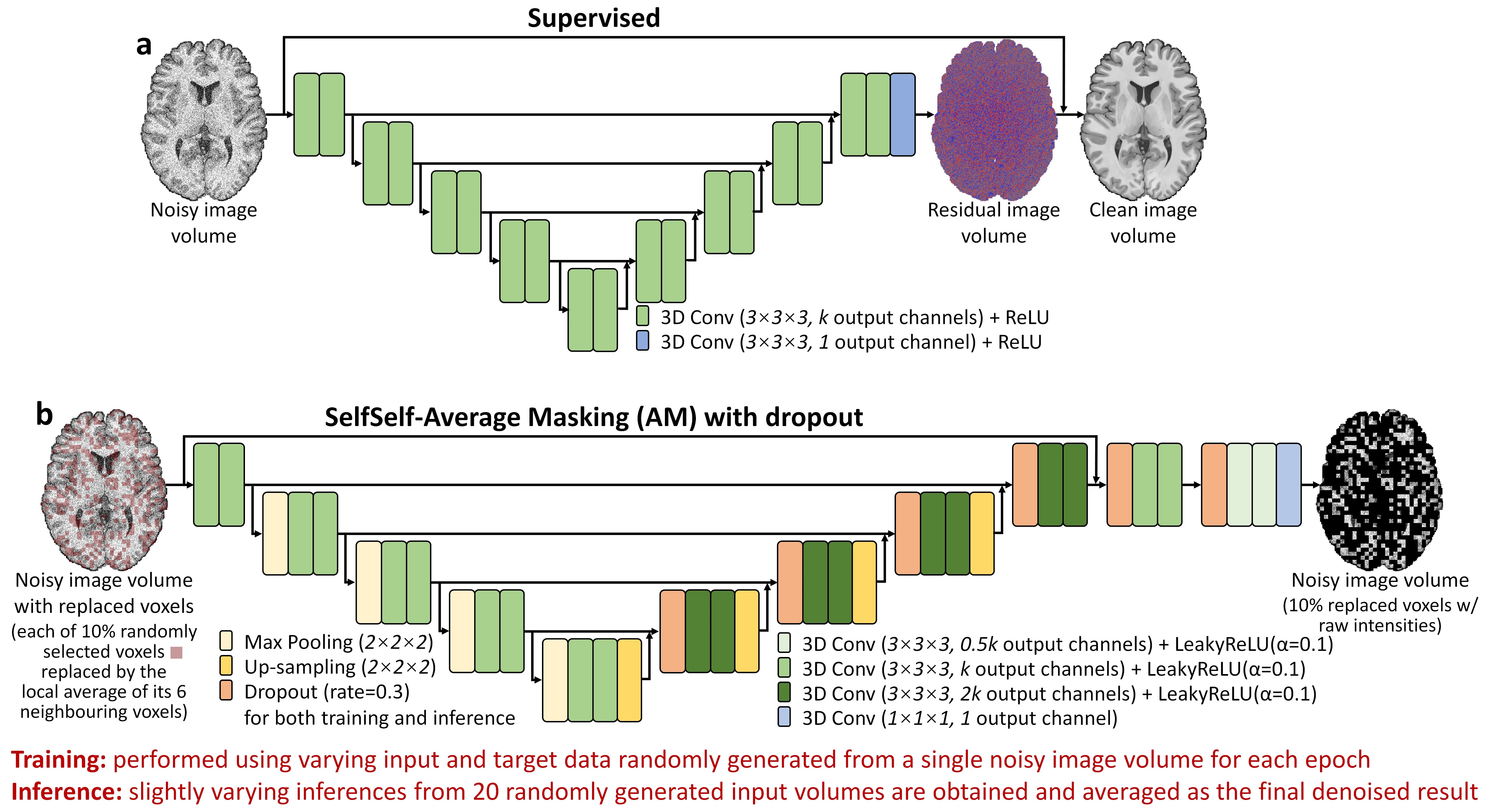
Denoising. For supervised denoising, a modified 3D U-Net¹⁹ that maps a noisy image volume to its residual compared to the high-SNR volume (Fig.1a) was trained on simulation data from 20 HCP subjects and directly applied to denoise Wave-CAIPI data. The pre-trained CNN was fine-tuned using either the data of a subject from the Skyra scanner or a subject from Prisma scanner, then was applied to denoising Wave-CAIPI data from the corresponding scanner.

For self-supervised denoising, Self2Self maps a noisy image with 10% randomly selected pixels set to zero to an image with only these 10% voxels with raw intensities, on which losses are calculated⁶. Here we extended Self2Self for volumetric data and to use average masking (Self2Self-AM), which sets each of 10% voxels to the average of its six neighboring voxels. Self2Self-AM employed a modified 3D U-Net with dropout layers enabled during both training and inference (Fig.1b). Slightly varying inferences from 20 randomly generated input volumes were averaged as the final result.

For each MGH subject, Self2Self-AM was trained for 1700 epochs (~1 minute/epoch), using a pair of input and target data randomly sampled from the Wave-CAIPI volume of this subject for each epoch. Moreover, the pre-trained Self2Self-AM CNN of an MGH subject was directly applied to denoise Wave-CAIPI data of other subjects, which was also fine-tuned for 17, 85 and 170 epochs using data from each MGH subject for reducing the training time of Self2Self-AM using transfer learning. Finally, Self2Self-AM was trained for 1700 epochs on the synthetic noisy data from an HCP subject and directly applied to denoise Wave-CAIPI data.

Training and validation were performed using the Tensorflow software with Adam optimizers (L2 loss) on 96×96×96 image blocks.

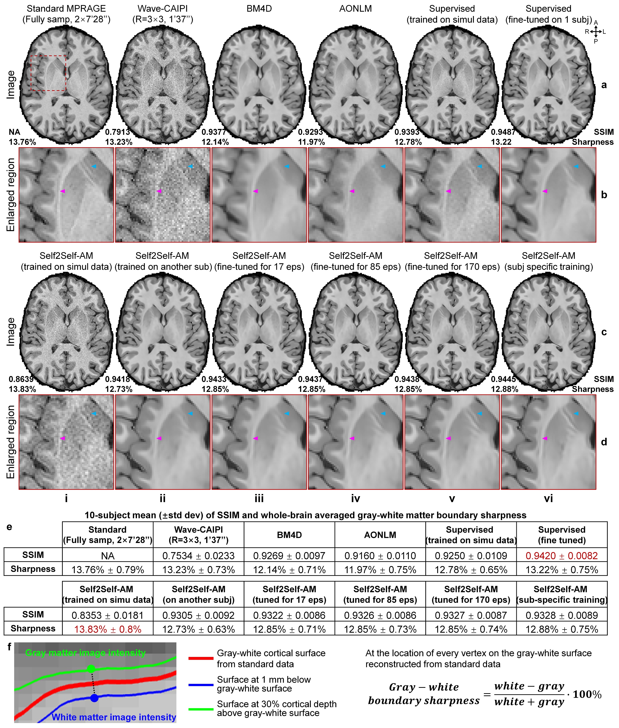
The Wave-CAIPI data were also denoised using state-of-the-art BM4D^20,21 and AONLM^22,23 algorithms.

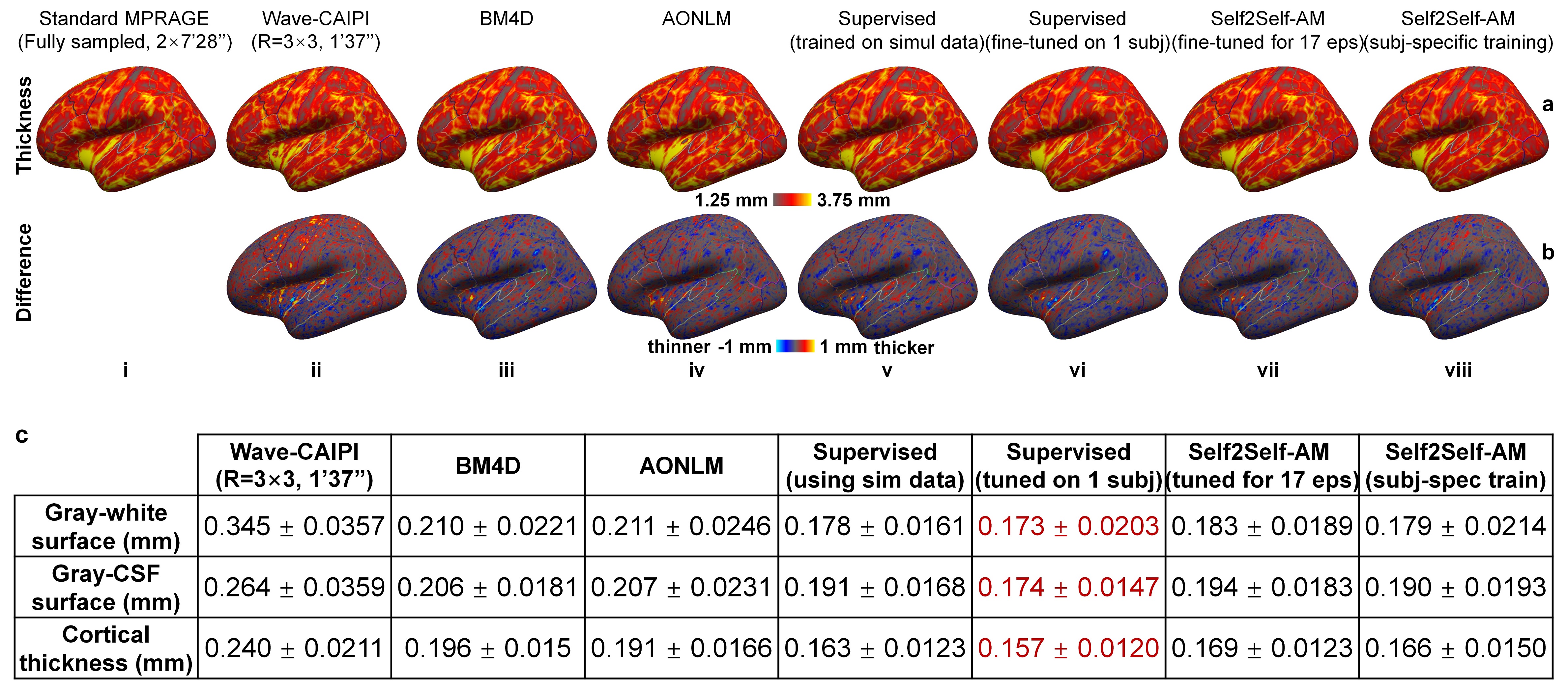
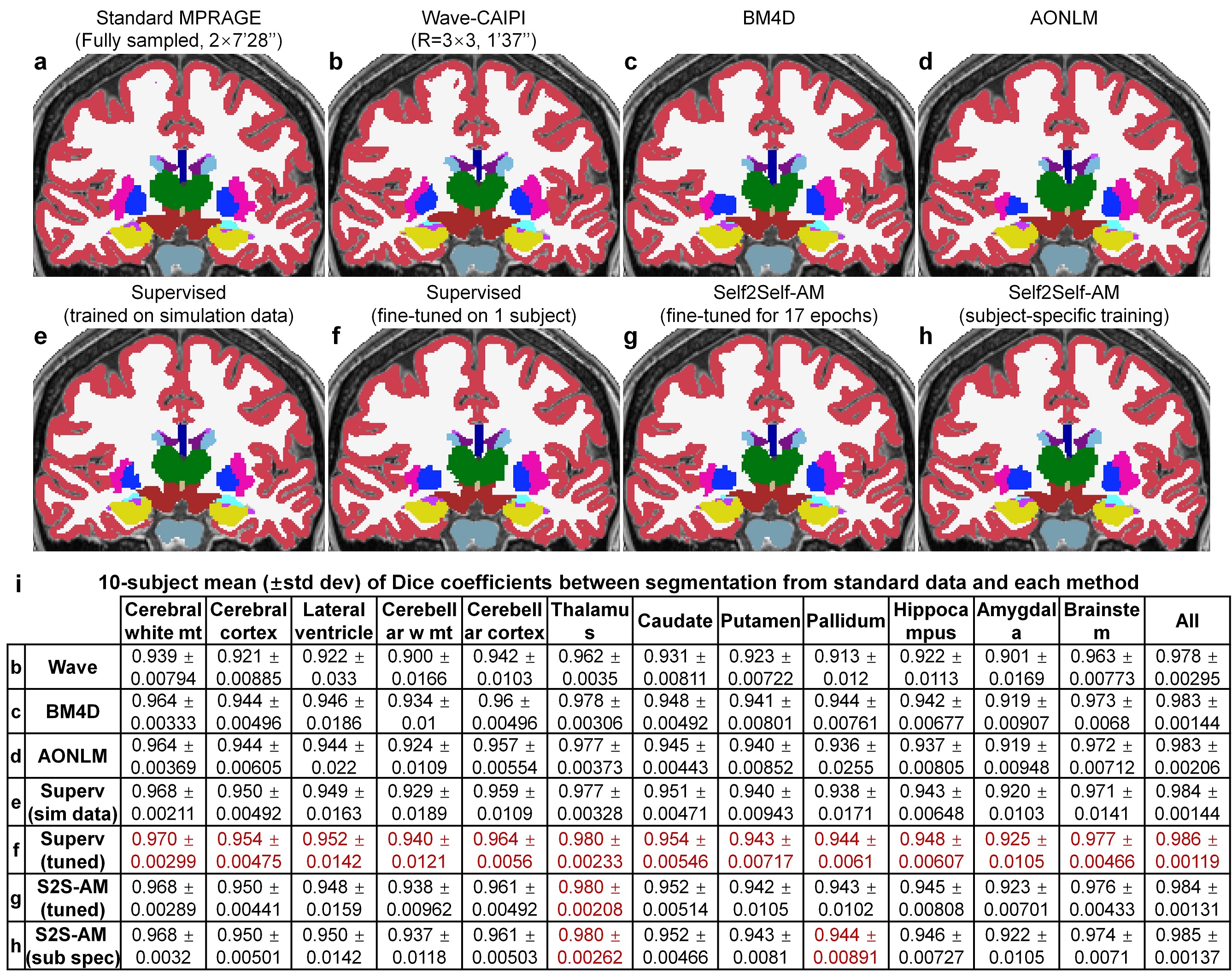
Evaluation. FreeSurfer reconstruction^12-14,24 was performed. The whole-brain averaged gray–white boundary sharpness (Fig.2f) was used to quantify image sharpness. The structural similarity index (SSIM) was used to quantify image similarity compared to standard images. The FreeSurfer longitudinal pipeline^11,25,26 was used to quantify the discrepancies between surface positioning and cortical thickness estimation^1,27. Dice coefficient was used to quantify the overlap of FreeSurfer’s “aseg” brain segments.

Results

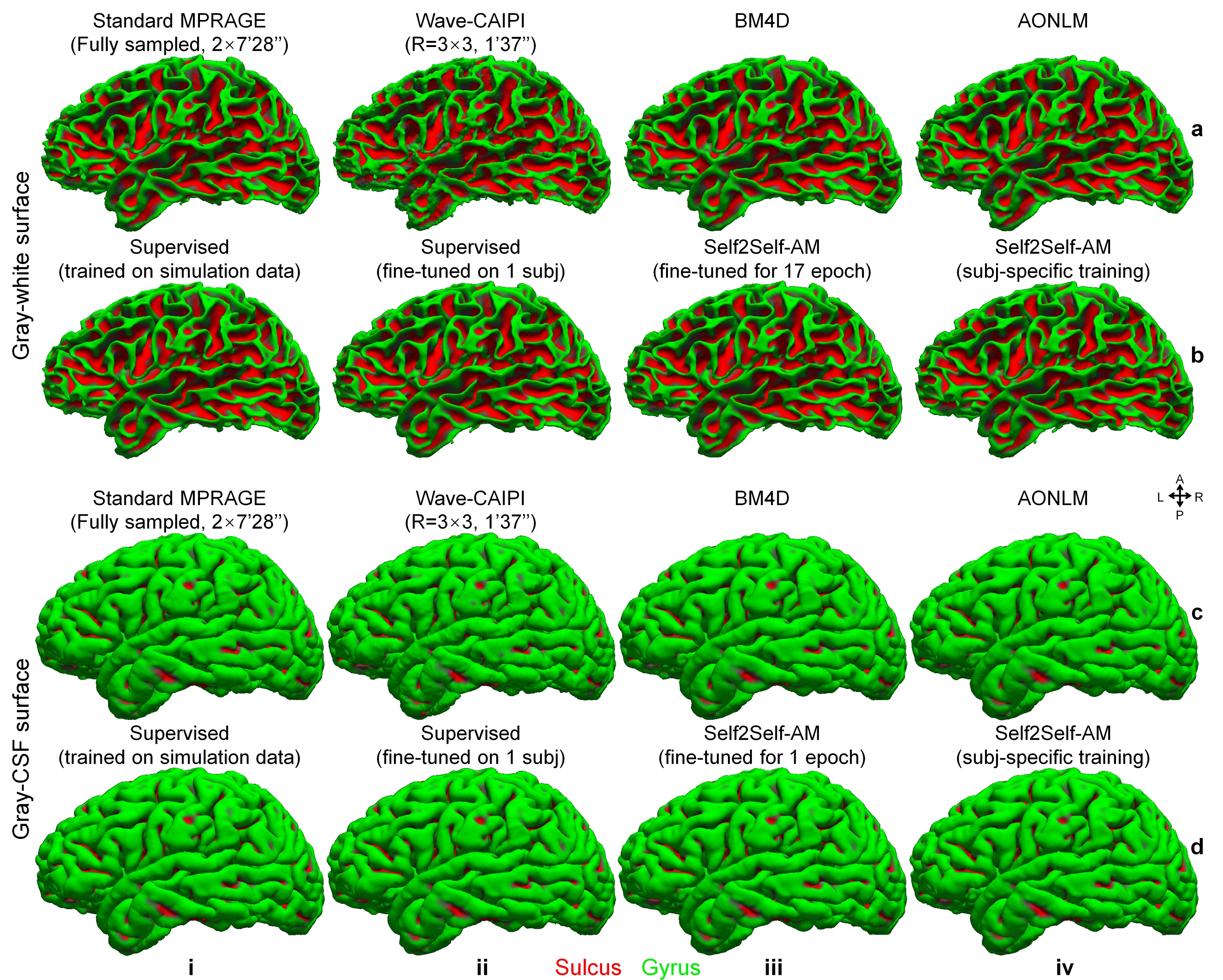
Supervised denoising trained on simulation data generalizes well to Wave-CAIPI data (Fig.2a,v) while our self-supervised denoising is less generalizable (Fig.2c,i). Supervised denoising after fine-tuning achieves the highest SSIM (Fig.2a,vi) while Self2Self-AM with subject-specific training achieves the second highest SSIM (Fig.2c,vi). Self2Self-AM by fine-tuning a pre-trained CNN for much shorter training time (Fig.2c,ii–v) results in slightly lower SSIM.

Cortical surfaces (Fig.3), cortical thickness (Fig.4) and brain segmentation (Fig.5) from all data are visually similar. Quantitatively, supervised denoising after fine-tuning achieves the lowest error in surface positioning and thickness estimation and highest Dice coefficients while Self2Self-AM with subject-specific training performs second best.

Discussion and Conclusion

CNNs without or with very limited high-SNR data or training data from many subjects denoise effectively. Supervised denoising with fine-tuning is recommended when high-SNR data of 1 subject are available. Self2Self-AM is recommended when high-SNR data are unavailable.

Acknowledgements

The T1w data at 0.7 mm isotropic resolution of 20 healthy subjects were provided by the Human Connectome Project, WU-Minn-Ox Consortium (Principal Investigators: David Van Essen and Kamil Ugurbil; U54-MH091657) funded by the 16 NIH Institutes and Centers that support the NIH Blueprint for Neuroscience Research; and by the McDonnell Center for Systems Neuroscience at Washington University. This work was supported by the National Institutes of Health (grant numbers P41-EB015896, P41-EB030006, U01-EB026996, U01 EB025162, S10-RR023401, S10-RR019307, S10-RR023043, R01-EB028797, R03-EB031175, K99-AG073506), the Athinoula A. Martinos Center for Biomedical Imaging and the NVidia Corporation for computing support. W.L. is an employee of Siemens Medical Solutions.

References

1. Tian Q, Zaretskaya N, Fan Q, et al. Improved cortical surface reconstruction using sub-millimeter resolution MPRAGE by image denoising. NeuroImage. 2021;233:117946.

2. Zhang K, Zuo W, Chen Y, Meng D, Zhang L. Beyond a gaussian denoiser: Residual learning of deep cnn for image denoising. IEEE Transactions on Image Processing. 2017;26(7):3142-3155.

3. Lehtinen J, Munkberg J, Hasselgren J, et al. Noise2Noise: Learning Image Restoration without Clean Data. The International Conference on Machine Learning. 2018:2965-2974.

4. Batson J, Royer L. Noise2self: Blind denoising by self-supervision. Paper presented at: International Conference on Machine Learning2019.

5. Krull A, Buchholz T-O, Jug F. Noise2void-learning denoising from single noisy images. The IEEE Conference on Computer Vision and Pattern Recognition. 2019:2129-2137.

6. Quan Y, Chen M, Pang T, Ji H. Self2self with dropout: Learning self-supervised denoising from single image. Paper presented at: Proceedings of the IEEE/CVF Conference on Computer Vision and Pattern Recognition2020.

7. Bilgic B, Gagoski BA, Cauley SF, et al. Wave‐CAIPI for highly accelerated 3D imaging. Magnetic resonance in medicine. 2015;73(6):2152-2162.

8. Polak D, Cauley S, Huang SY, et al. Highly‐accelerated volumetric brain examination using optimized wave‐CAIPI encoding. Journal of Magnetic Resonance Imaging. 2019;50(3):961-974.

9. Polak D, Setsompop K, Cauley SF, et al. Wave‐CAIPI for highly accelerated MP‐RAGE imaging. Magnetic Resonance in Medicine. 2018;79(1):401-406.

10. Longo MGF, Conklin J, Cauley SF, et al. Evaluation of Ultrafast Wave-CAIPI MPRAGE for Visual Grading and Automated Measurement of Brain Tissue Volume. American Journal of Neuroradiology. 2020;41(8):1388-1396.

11. Reuter M, Rosas HD, Fischl B. Highly accurate inverse consistent registration: a robust approach. NeuroImage. 2010;53(4):1181-1196.

12. Fischl B, Sereno MI, Dale AM. Cortical surface-based analysis: II: inflation, flattening, and a surface-based coordinate system. NeuroImage. 1999;9(2):195-207.

13. Dale AM, Fischl B, Sereno MI. Cortical surface-based analysis: I. Segmentation and surface reconstruction. NeuroImage. 1999;9(2):179-194.

14. Fischl B. FreeSurfer. NeuroImage. 2012;62(2):774-781.

15. Modat M, Ridgway GR, Taylor ZA, et al. Fast free-form deformation using graphics processing units. Computer Methods and Programs in Biomedicine. 2010;98(3):278-284.

16. Modat M, Cash DM, Daga P, Winston GP, Duncan JS, Ourselin S. Global image registration using a symmetric block-matching approach. Journal of Medical Imaging. 2014;1(2):024003-024003.

17. Glasser MF, Sotiropoulos SN, Wilson JA, et al. The minimal preprocessing pipelines for the Human Connectome Project. NeuroImage. 2013;80:105-124.

18. Glasser MF, Smith SM, Marcus DS, et al. The human connectome project's neuroimaging approach. Nature Neuroscience. 2016;19(9):1175-1187.

19. Falk T, Mai D, Bensch R, et al. U-Net: deep learning for cell counting, detection, and morphometry. Nature Methods. 2019;16(1):67-70.

20. Dabov K, Foi A, Katkovnik V, Egiazarian K. Image denoising by sparse 3-D transform-domain collaborative filtering. IEEE Transactions on Image Processing. 2007;16(8):2080-2095.

21. Maggioni M, Katkovnik V, Egiazarian K, Foi A. Nonlocal transform-domain filter for volumetric data denoising and reconstruction. IEEE Transactions on Image Processing. 2012;22(1):119-133.

22. Coupé P, Yger P, Prima S, Hellier P, Kervrann C, Barillot C. An optimized blockwise nonlocal means denoising filter for 3-D magnetic resonance images. IEEE transactions on medical imaging. 2008;27(4):425-441.

23. Manjón JV, Coupé P, Martí‐Bonmatí L, Collins DL, Robles M. Adaptive non‐local means denoising of MR images with spatially varying noise levels. Journal of Magnetic Resonance Imaging. 2010;31(1):192-203.

24. Fischl B, Van Der Kouwe A, Destrieux C, et al. Automatically parcellating the human cerebral cortex. Cerebral Cortex. 2004;14(1):11-22.

25. Reuter M, Schmansky NJ, Rosas HD, Fischl B. Within-subject template estimation for unbiased longitudinal image analysis. NeuroImage. 2012;61(4):1402-1418.

26. Reuter M, Fischl B. Avoiding asymmetry-induced bias in longitudinal image processing. NeuroImage. 2011;57(1):19-21.

27. Zaretskaya N, Fischl B, Reuter M, Renvall V, Polimeni JR. Advantages of cortical surface reconstruction using submillimeter 7 T MEMPRAGE. NeuroImage. 2018;165:11-26.

Figures

Figure 1. Network architecture. For supervised learning, the CNN is a modified U-Net without max pooling and up-sampling layers, with the residuals between the noisy and high-SNR image volume as the training target. For Self2Self with average masking (AM), the CNN is a modified U-Net with dropout layers which behave during both training and inference. Each of 10% randomly selected voxels of the input noisy image volume is replaced by the average of its 6 neighbouring voxels. The target is a volume only with these 10% replaced voxels with raw intensities, on which L2 losses are computed.

Figure 2. Image results. Exemplar image slices from standard data, Wave-CAIPI data and denoised Wave-CAIPI data (a, c) of a representative subject, with magnified views of basal ganglia (b, d). The structural similarity index (SSIM) compared to standard images and whole-brain averaged vertex-wise gray–white matter boundary sharpness (f) are listed to quantify image quality. The arrowheads highlight the claustrum and caudolenticular gray bridges with fine textures with fine textures. The group means (±std dev) of SSIM and sharpness are listed in the table (e).

Figure 3. Cortical surfaces. Gray–white interface surfaces (a, b) and gray–cerebrospinal fluid (CSF) interface surfaces (c, d) reconstructed from standard, Wave-CAIPI and denoised Wave-CAIPI data using FreeSurfer of a representative subject.

Figure 4. Cortical thickness. Left-hemispheric vertex-wise cortical thickness estimates from different data (a) and their difference (b) compared to those from standard data (a, i) of a representative subject, displayed on inflated surface representations. The group means (±std dev) of the whole-brain averaged absolute displacement/difference of the gray–white surface, gray–cerebrospinal fluid (CSF) surface and cortical thickness (c) estimated from different data compared to standard data are listed (d).

Figure 5. Brain segmentation. Exemplar image slices of brain structures segmented using different data (FreeSurfer’s aseg) of a representative subject (a–h). The group means (±std dev) of Dice coefficients between the segments from different data and standard data are listed for 12 brain structures and all of them combined are listed (i).

Proc. Intl. Soc. Mag. Reson. Med. 30 (2022)

4811

DOI: https://doi.org/10.58530/2022/4811