Introduction

Metabolite concentrations can be determined by MRS spectral fitting, commonly conducted by fitting parametric model spectra to the data [1]. The fitting is often complicated by spectral overlaps, especially for those weakly represented metabolites. There are also unknown or not well-defined signals originating from macromolecules and/or lipids which give rise to complex backgrounds and further confound the fitting process. Multi echo techniques such as JPRESS consist of both short and long echoes and provide more diversified information for spectral fitting than techniques based on a single echo. However, fitting multi echo data is more challenging because signals attenuate with increasing echo time (TE) due to T2 relaxation, and the macromolecule background also varies across the echoes. Recently, artificial neural networks have been increasingly applied to MRS including spectral quantification. Lee et. al. [2] presented a convolutional neural network (CNN) architecture that learns to map the input data in the frequency domain to the target spectra that are a linear combination of basis spectra. Gurbani et. al. [3] incorporated a convolutional encoder into parametric model fitting. We present here a novel neural network architecture that directly maps the time domain JPRESS input onto metabolite concentrations.

Methods

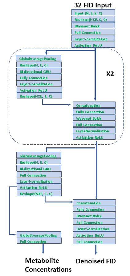
The proposed neural network architecture is shown schematically in Fig. 1. The input consists of 32 echo FIDs in the time domain. The front end after the data reshaping is a Wavenet block [4]. It takes 2-channel input (real and imaginary) and creates hidden representations generalized for all echoes with 128 dimensions. The outputs are split into two branches. One branch is averaged by global average pooling and sent to a bi-directional gated recurrent unit (GRU) block where the representations for individual 32 echoes are integrated and then concatenated with the other branch of output from the Wavenet. This process repeats twice and proceeds to the final layers, yielding denoised 32 echo FIDs and metabolite concentrations. The two tasks of denoising and predicting metabolite concentrations are combined to facilitate training. 18 metabolite basis spectra including water were generated using quantum mechanics simulations [5]. The simulation mimics the JPRESS sequence implemented on a GE 3T scanner. The JPRESS sequence has 32 echoes with TE starting from 35 ms and incrementing by 6 ms after each echo. The simulated spectra of individual metabolites were combined to create the training and evaluation datasets. The concentration of each metabolite is random and uniformly distributed, spanning from zero to twice of the reported in vivo values measured in healthy subjects [6]. The resonant frequency of each metabolites and water was randomly varied with uniform distributions over a specified range (0-20 Hz for water; 0-5 Hz for metabolites relative to water). Line-broadening was applied to the basis spectra with a random distribution over a range of 0-5 Hz, and T2s was varied randomly from the T2 values of the basis spectra by ± 50 ms. The phases were also changed randomly over 0-360o. For each echo, up to three extraneous peaks with linewidth in the range of 20-30 Hz and random phases were generated. The amplitude of extraneous signals decays with increasing echo number, mimicking transverse relaxation. These extraneous signals were added to the data to create adversarial perturbations, forcing the model to discard undesired features such as the macromolecule background during training. Finally, random noise was injected into the data. The final training dataset includes 40000 samples. An additional dataset containing 2000 samples were created in the same fashion for evaluation.

Results

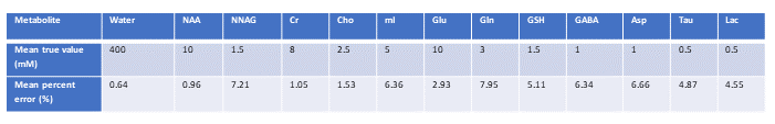
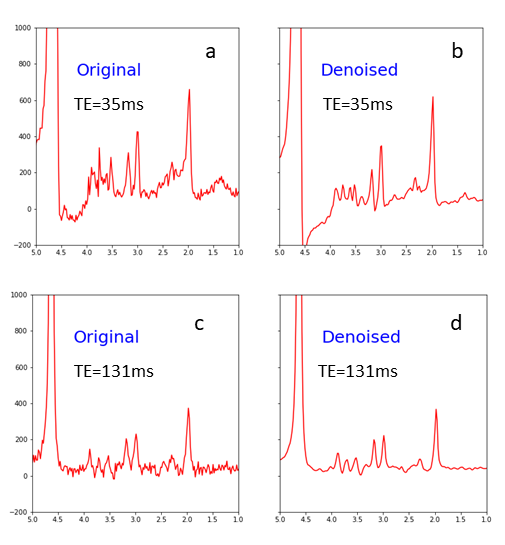
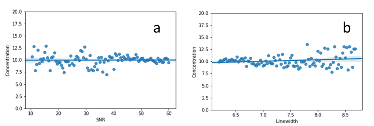
The predication errors from testing by the evaluation dataset are given in Table 1. Fig. 2 shows comparison between original in vivo spectra and the spectra denoised by the model; only the first echo (TE = 35ms) and 16th echo (TE = 131ms) are displayed. Note that macromolecule signals in the vicinity of 2.5 ppm and 3.5 ppm are reduced for TE = 35 ms (Fig. 2a vs. 2b); a large increase in SNR is seen for TE = 131 ms (Fig. 2c vs. 2d). The SNR (defined as the ratio of NAA acetyl peak height to noise level) for TE-averaged spectra was increased by 2.8-fold on average. As shown in Fig. 3 no significant correlations for the mean predicted Glu concentrations were found as the in vivo data were progressively degraded by noise injection and line broadening accompanied by increased standard deviations. The straight lines and shaded areas from Bayesian linear regression were also shown in Fig. 3.

Discussion and Conclusion

Metabolites have fixed resonance frequencies relative to each other, allowing a convolutional kernel to extract the spectral features of individual metabolites in the time domain and generate representations that map the metabolite concentrations (with 128 dimensions in this study). Unlike wavelet transformations which have convolutional kernels given in analytical forms, the convolutional neural network learns the kernels itself from training. GRU is a recurrent neural network which can connect different echoes in the time domain and creates a single representation for the entire echo series. In conclusion, this study shows a model trained using simulated spectral data can successfully predict in vivo metabolite concentrations from multi-echo JPRESS data.

Acknowledgements

No acknowledgement found.