Purpose

Banding artifacts in balanced steady state free precession (bSSFP) images can be resolved by applying radiofrequency phase cycling and taking a Fourier transform across the phases, resulting in signal modes (1). The steady state signal and its modes have been analytically described (2,3). Post-processing of those modes can be used to augment image contrast (4). Ellipse fitting in the complex signal plane allows calculation of tissue properties such as T₁ and T₂ (5). Unfortunately, the scan time increases linearly with the amount of phase cycles measured, hindering clinical adoption of this sequence. This paper aims to reduce the amount of phase cycles that need to be acquired by employing the aforementioned signal model in an iterative reconstruction.

Methods

Iterative reconstruction
Let s be the acquired signal in one voxel. The fast Fourier transform (fft) of the signal, S, is taken such that initial estimates of the modes M⁽⁰⁾, M⁽¹⁾, and M^(-1) can be obtained:
$$M^{(p)} = |S^{(p)}|$$
Following equations 11 and 12 in (6), initial estimates for the transceive phase, $$$\phi$$$, and off-resonance, $$$\theta$$$, can also be obtained:
$$\theta = arg(\frac{S^{(1)}}{S^{(-1)}})+\pi$$
$$\phi = arg(S^{(1)} \cdot S^{(-1)}) /2$$
Note that these estimates may suffer from aliasing if the number of acquired phase cycles is low.

From equation 2 in (3) it follows that higher-order modes can be described in terms of M⁽⁰⁾, M⁽¹⁾ and M^(-1):
$$M(n)=\begin{cases}\frac{M^{(1)n}}{M^{(0)n-1}} & n>1 \\ \frac{M^{(-1)} \cdot M^{(1)-n-1}}{M^{(0)-n-1}} & n<-1\end{cases}$$
Following equation 7 in (6), and ignoring the aliasing terms, the Fourier transform of the signal, S, can be fully described in terms of M⁽⁰⁾, M⁽¹⁾, M^(-1), $$$\theta$$$ and $$$\phi$$$:
$$S^{(p)} = e^{i \phi} e^{i \theta/2} e^{i p \theta} M^{(p)}$$

After calculating M⁽⁰⁾, M⁽¹⁾, M^(-1), $$$\theta$$$ and $$$\phi$$$: from measured data, a set amount of synthetic higher order modes are calculated to increase the number of modes by a factor k. We then switch back to the measurement domain using an inverse fft on the synthetic mode data. Now we obtain synthetic data with the number of phase cycles increased by a factor k. Next, we correct the synthetic data by inserting the measured data on every k-th phase cycle. Then, we transform the data to the mode domain, calculate new estimates of M⁽⁰⁾, M⁽¹⁾, M^(-1), $$$\theta$$$ and $$$\phi$$$ from the corrected synthetic dataset and use these to generate a new synthetic dataset. We iterate between creating synthetic datasets and correcting them by inserting measured data, until convergence.

In-silico validation
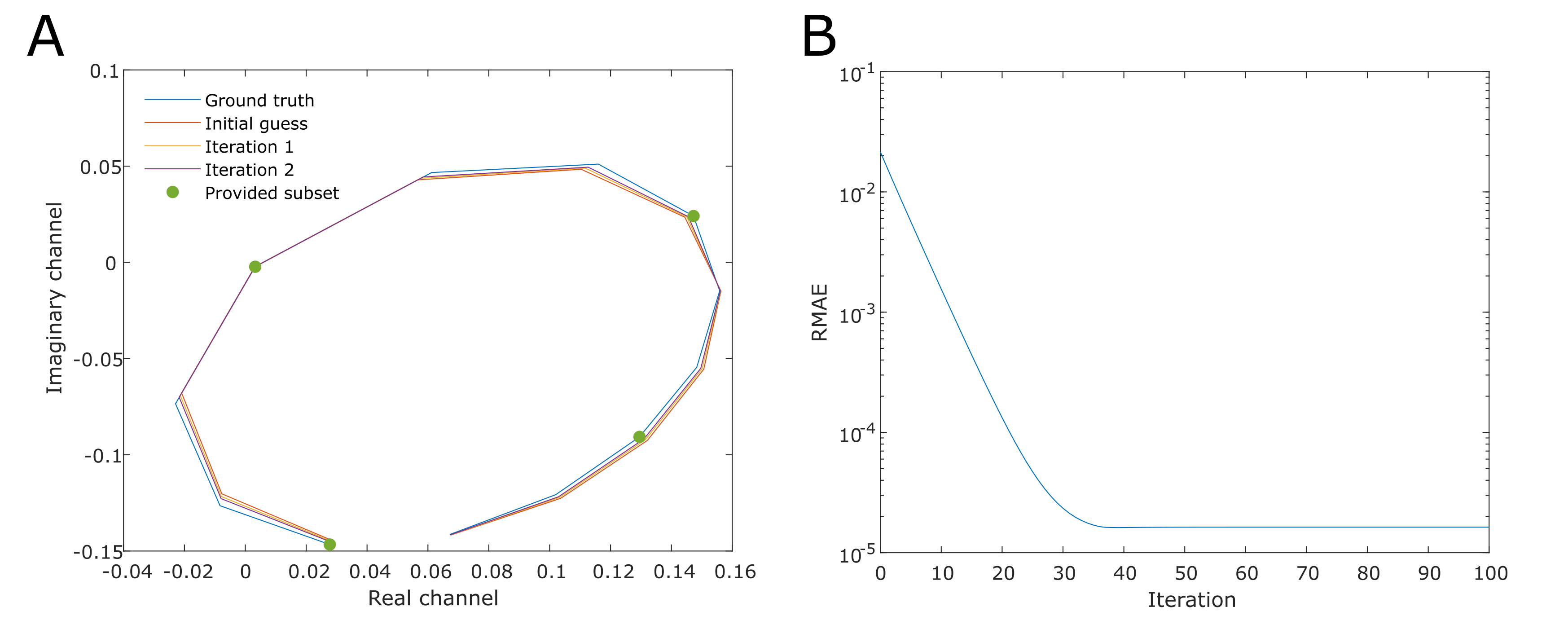
A synthetic signal was generated using tissue properties T₁ = 2000 ms, T₂ = 200 ms, and sequence parameters FA 35$$$^{\circ}$$$, TR 5 ms, $$$\Delta f_0$$$ 50 Hz, $$$\phi$$$ 10$$$^{\circ}$$$. 12 equidistant phase cycles were simulated as ground truth. A subset of 4 equidistant phase cycles (#1,4,7,10) was provided as input for the iterative reconstruction described above. Every iteration the relative mean absolute error (RMAE) was calculated between the predicted and true values for this subset. The algorithm was run for 100 iterations to observe its convergence. The final result was evaluated by calculating the RMAE over the full predicted dataset against ground truth.

Phantom validation
The Eurospin II TO5 phantom (Diagnostic Sonar LTD, Livingston, Scotland) was imaged on a 1.5T Philips Ingenia machine. We acquired a 3D phased-cycled (PC-) bSSFP with 12 equidistant phase cycles over 360$$$^{\circ}$$$ (9.06 Hz offset between phases), TR 9.2 ms, TE 4.6 ms, FA 35$$$^{\circ}$$$, readout bandwidth 430 Hz/pix, acquired resolution 1.2x1.2x2 mm³, reconstructed to 0.7x0.7x2 mm³, with a compressed sense factor of 3 in 53 s per phase cycle (11 min total scan time).

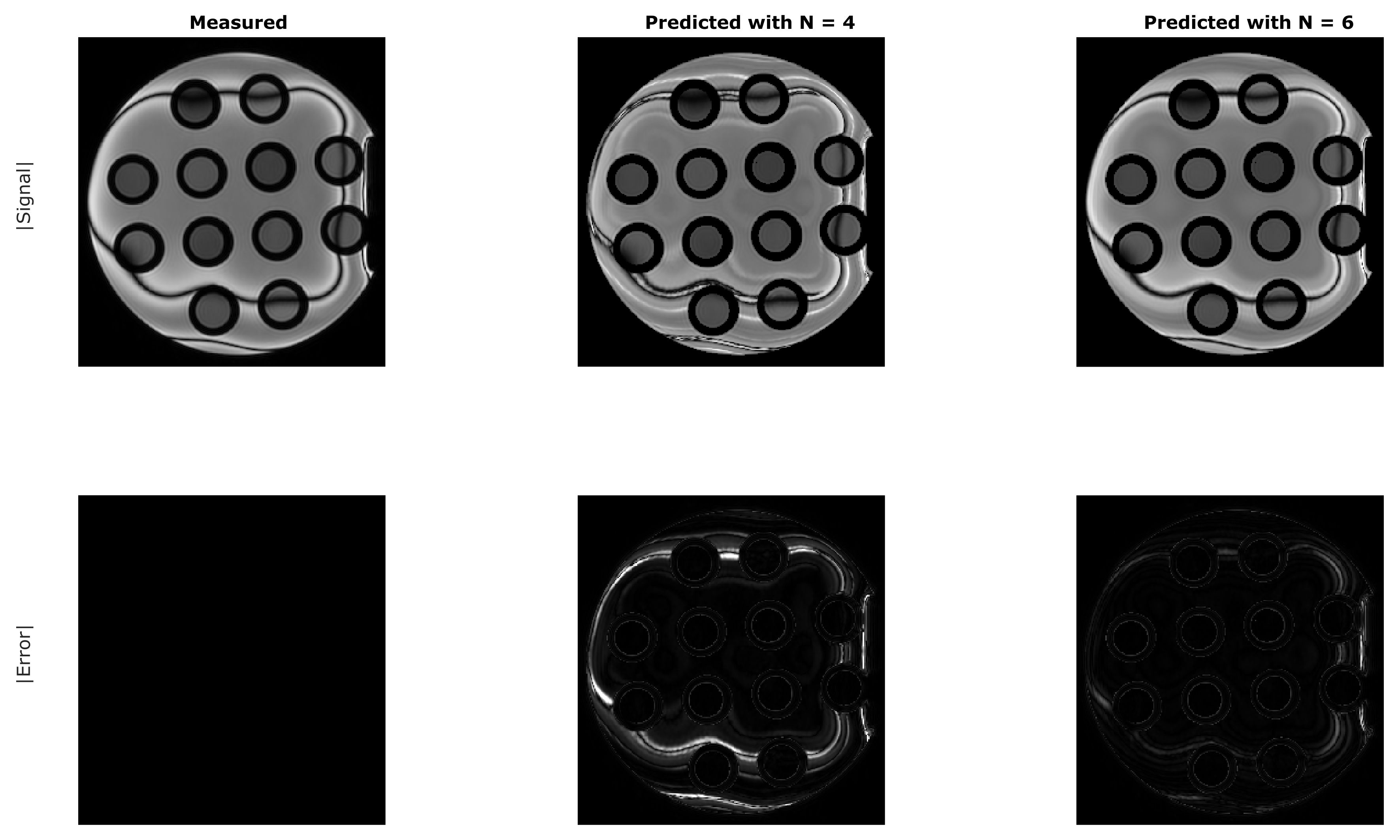
Like in the in-silico validation, the full dataset was predicted from a subset of either 6 equidistant phase cycles (#1,3,5,7,9,11) or 4 cycles (#1,4,7,10). The algorithm was run until the RMAE no longer improved (difference < 0.01%). The final results were compared against the full dataset both visually and by calculating the RMAE in a region inside the phantom tubes.

Results

In-silico
Figure 1 shows the results of the in-silico validation. The algorithm converged after 44 iterations. The RMAE of the final result was 0.0045%.

Phantom
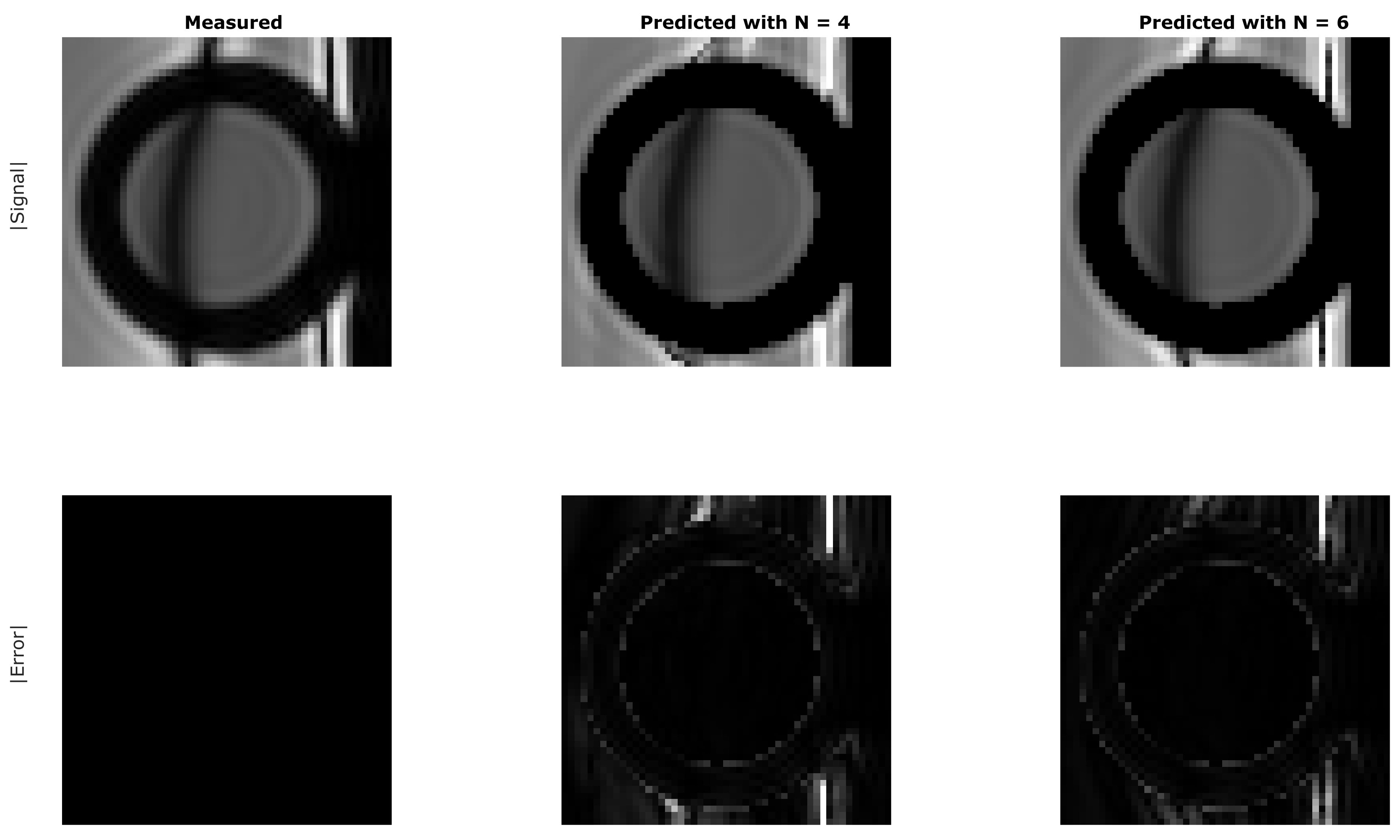
Figure 2 shows the result for a single slice of the phantom at a single predicted phase cycle, #2, for both N = 4 and N = 6 phase cycles. Figure 3 shows the same data, but a zoom-in on a single tube. Most errors occur in the body of the phantom, but due to the long T₁ and T₂ of this area, steady state may never be reached there. Further analysis focused on the tubes only and the RMAE in the tubes was 3.20% when predicted with 6 phase cycles, 4.21% when predicted with 4 phase cycles. Figure 4 shows the predicted modes for a single tube from 4 phase cycles versus the measured modes at 4 and 12 phase cycles, indicating the improvement achieved by iterative reconstruction.

Conclusion

We have developed an iterative reconstruction algorithm to predict additional phase cycles in PC-bSSFP. Preliminary validation shows good agreement in phantom tubes with T₁ and T₂ values in the physiological range. Future work will focus on a more extensive validation in-vivo.

Acknowledgements

No acknowledgement found.