4755
Deep-Learning-regularized Single-step Quantitative Susceptibility Mapping (QSM) Quantification1Department of Diagnostic Radiology, The University of HongKong, Hong Kong, China
Synopsis
We develop a deep-learning-regularized single-step QSM quantification to generate QSM directly from the total phase map. A deep-learning-regularized dipole inversion network, named POCSnet, was deployed to a single-step QSM (SS-POCSnet) network, which combined a variable-SHARP (VSHARP) and the POCSnet. Meanwhile, SS-POCSnet showed improved accuracy compared with conventional single-step QSM methods. We also demonstrated the generalizability of SS-POCSnet on different datasets in vivo.
Introduction
Quantitative susceptibility mapping (QSM) is frequently used in the diagnosis of neurological diseases1. However, conventional QSM quantification required background field removal and dipole inversion steps2,3. Single-step QSM quantification methods, such as SS-L2-QSM4 and total field inversion (TFI)5, were developed to reduce error propagation in the two-step approach. Nevertheless, conventional single-step QSM methods had many parameters to tune, which might limit their applications. Recently, deep learning-based methods solved ill-posed MRI reconstruction and quantification problems, achieving superior performance compared with the conventional regularizations. A single-step deep learning model, autoQSM, generated QSM from the total field map directly using naïve feedforward model6. Additionally, the LPCNN7 and MoDL-QSM8 combined the fidelity term with a proximal network for dipole inversion. However, no deep learning model with data fidelity term was used in single-step QSM quantification. In this study, we proposed a deep-learning-regularized single-step QSM quantification, named SS-POCSnet. We evaluated the model performance on different datasets with varied matrix sizes and resolutions.Methods
We firstly trained a deep-learning-regularized dipole inversion network, named POCSnet. Then we deployed the deep learning regularization in a neural network called single-step POCSnet (SS-POCSnet). SS-POCSnet regularized both the VSHARP2 and dipole inversion terms, mitigating the tissue phase and susceptibility underestimation. In POCSnet, the closed-form solution of susceptibility map was iteratively calculated as follows:χ =(FHDHDF+λ1I)-1FHDF𝝋+ λ1(FHDHDF+λ1I)-1χnet (1)
where 𝝋 is phase map, D the dipole model in Fourier domain, and F the Fourier transform, χnet the neural network (i.e., V-Net here) output, and ƛ1 the regularization parameter. (Figure 1a).In SS-POCSnet, the minimization problem for VSHARP2 with deep-learning regularization is
𝝋local =argmin𝝋local½(MiFHCiF(𝝋local-𝝋total))2+λ2/2(𝝋local-𝝋net)2 (2)
where M the eroded brain mask, C the SMV kernel in Fourier domain, ƛ2 the regularization parameter, i index for varied radii SMV kernels in VSHARP method, and tissue phase from the neural network 𝝋net can be derived as below.
𝝋net=FHDFχnet (3)
Eq.2 is solved using a conjugate gradient algorithm (CG), and the solution is fed into Eq. 1 to update χk. The parameters are ƛ1 = ƛ2 = 0.1, max iterations = 5, number of CG = 3. SMV kernels of 1, 5, 12 mm were used (Figure 1b).
For training POCSnet, 950 paired susceptibility maps and phase maps in matrix size 64×64×64 and resolution 0.86×0.86×1.00 mm3/pixel were simulated. For model testing, one COSMOS data (matrix size = 160×160×160, resolution = 1.06×1.06×1.06 mm3/pixel) from the 2016 QSM reconstruction challenge9, and three patient datasets (QSM acquisition: matrix size = 704 × 704 × 135, nominal resolution = 0.3267 × 0.3267 × 1.0 mm3/pixel; T1w image: matrix size = 800 × 800 × 25, and resolutions = 0.29 × 0.29 × 5.5 mm3/pixel and T2w-FLAIR: matrix size = 512 × 512 × 330, and resolution = 0.49 × 0.49 × 0.56 mm3/pixel) were applied. In addition, SS-L2-QSM4 and autoQSM6 were configured with reasonable parameters for comparison. And ROIs in deep grey matters of COSMOS were segmented for model analysis.
The NRMSE was used for training POCSnet. Other parameters are ‘ADAM’ optimizer with beta = (0.9, 0.99), number of epochs = 198, and learning rate = 2 × 10⁻⁵. As data augmentation, adjacent batches were randomly scaled and summed during model training. For model inference, the pre-trained POCSnet model was applied to SS-POCSnet directly, without retraining the model. TensorFlow v2.2.0 and Keras v2.4.3 were used on a GPU server equipped with four NVIDIA 3090 Ti GPUs, 16 GB RAM, and 8-core Intel Xeon CPU. It took around 8 hours to train POCSnet on one GPU.
Results
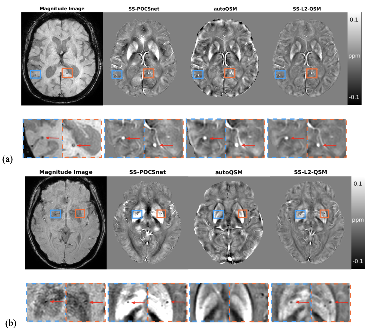
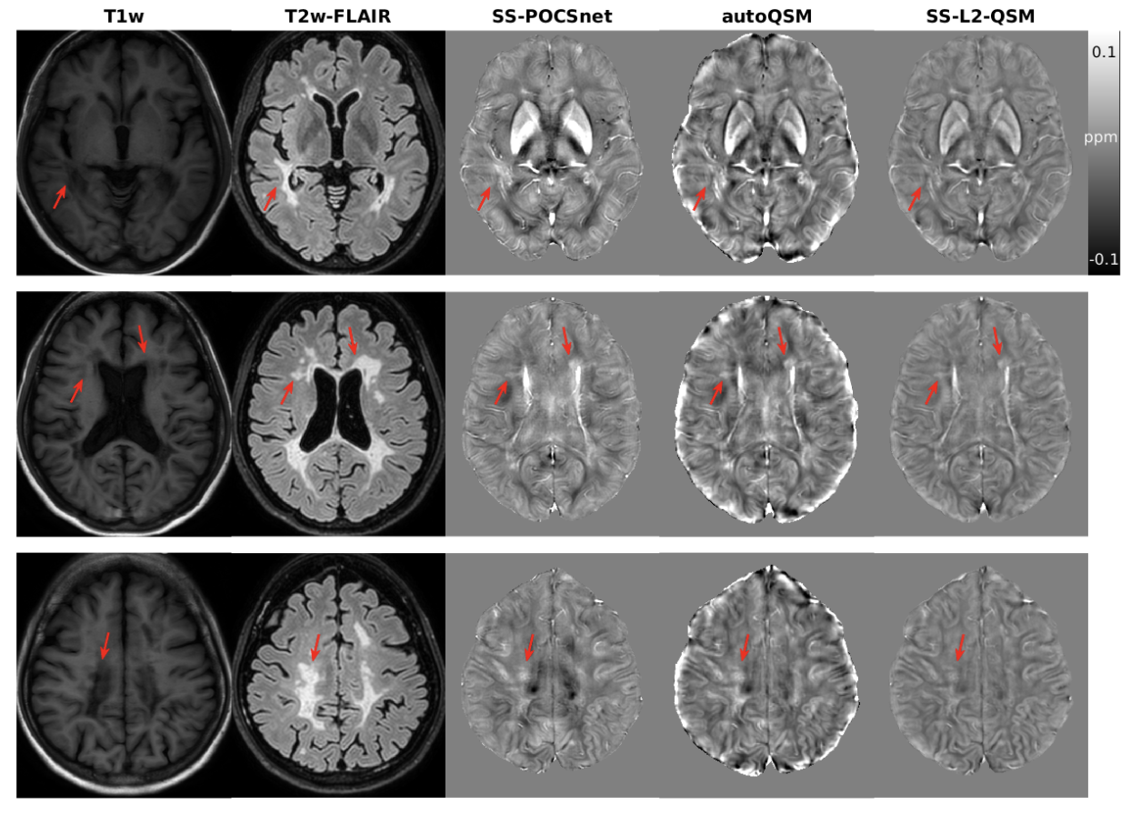
SS-POCSnet had the best quantitative results among methods evaluated (in Table 1). VSHARP+SS-POCSnet and SS-POCSnet were both able to delineate detailed anatomical structures. In Figure 2, the image profile of SS-POCSnet was closer to that of COSMOS compared with the profiles of other methods and the underestimations were reduced in results from SS-POCSnet. Figures 3 compared QSM maps generated by these methods, from patients with CMBs and calcifications. SS-POCSnet provided better image contrasts with generally reduced residual background and underestimations. Moreover, the CMBs were expected to be hyperintensities on QSM and two calcification balls were not visible in results from autoQSM. Finally, MS lesions were indicated by arrows and more detectable on results from SS-POCSnet.Conclusion
Deep-learning-regularized single-step QSM quantification can mitigate underestimating susceptibility values in deep brain nuclei and generate a QSM volume in ~40 seconds.Acknowledgements
This work is supported by Hong Kong Health and Medical Research Fund 07182706 and 06172916.References
1. Wang Y, Spincemaille P, Liu Z, et al. Clinical quantitative susceptibility mapping (QSM): Biometal imaging and its emerging roles in patient care. J Magn Reson Imaging. Oct 2017;46(4):951-971. doi:10.1002/jmri.25693.
2. Ozbay PS, Deistung A, Feng X, Nanz D, Reichenbach JR, Schweser F. A comprehensive numerical analysis of background phase correction with V-SHARP. Nmr in Biomedicine. Apr 2017;30(4)doi:ARTN e355010.1002/nbm.3550.
3. Wei HJ, Dibb R, Zhou Y, et al. Streaking artifact reduction for quantitative susceptibility mapping of sources with large dynamic range. Nmr in Biomedicine. Oct 2015;28(10):1294-1303. doi:10.1002/nbm.3383.
4. Bilgic B, Langkammer C, Wald1 LL, Setsompop K. Single-step QSM with fast reconstruction. Third International Workshop on MRI Phase Contrast & Quantitative Susceptibility Mapping. 2014.
5. Liu Z, Kee Y, Zhou D, Wang Y, Spincemaille P. Preconditioned total field inversion (TFI) method for quantitative susceptibility mapping. Magn Reson Med. Jul 2017;78(1):303-315. doi:10.1002/mrm.26331.
6. Wei HJ, Cao S, Zhang YY, et al. Learning-based single-step quantitative susceptibility mapping reconstruction without brain extraction. Neuroimage. Nov 15 2019;202doi:UNSP 11606410.1016/j.neuroimage.2019.116064.
7. Lai KW, Aggarwal M, van Zijl P, Li X, Sulam J. Learned Proximal Networks for Quantitative Susceptibility Mapping. Med Image Comput Comput Assist Interv. Oct 2020;12262:125-135. doi:10.1007/978-3-030-59713-9_13
8. Feng R, Zhao J, Wang H, et al. MoDL-QSM: Model-based Generative Adversarial Deep Learning Network for Quantitative Susceptibility Mapping. arXiv:210108413v1. 2021;
9. Langkammer C, Schweser F, Shmueli K, et al. Quantitative susceptibility mapping: Report from the 2016 reconstruction challenge. Magnet Reson Med. Mar 2018;79(3):1661-1673. doi:10.1002/mrm.26830
Figures
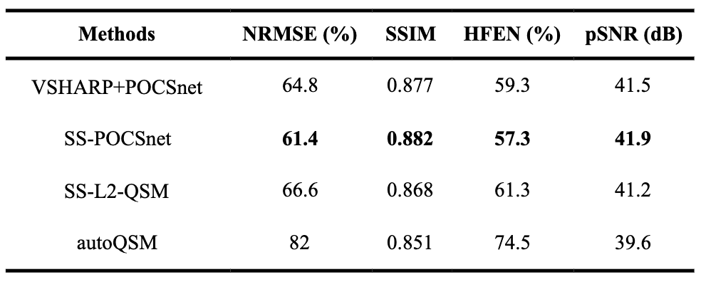
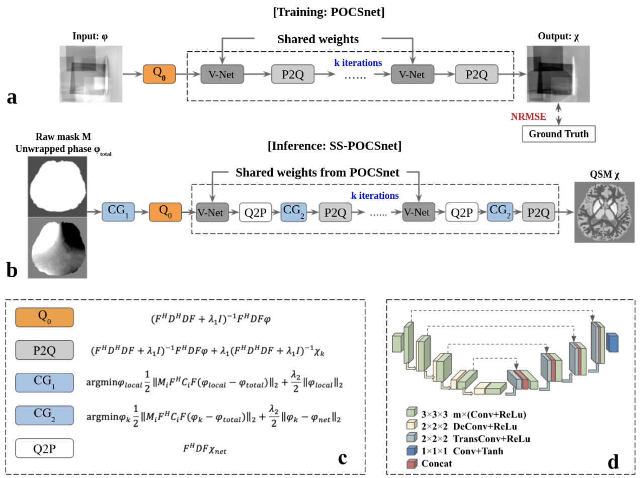
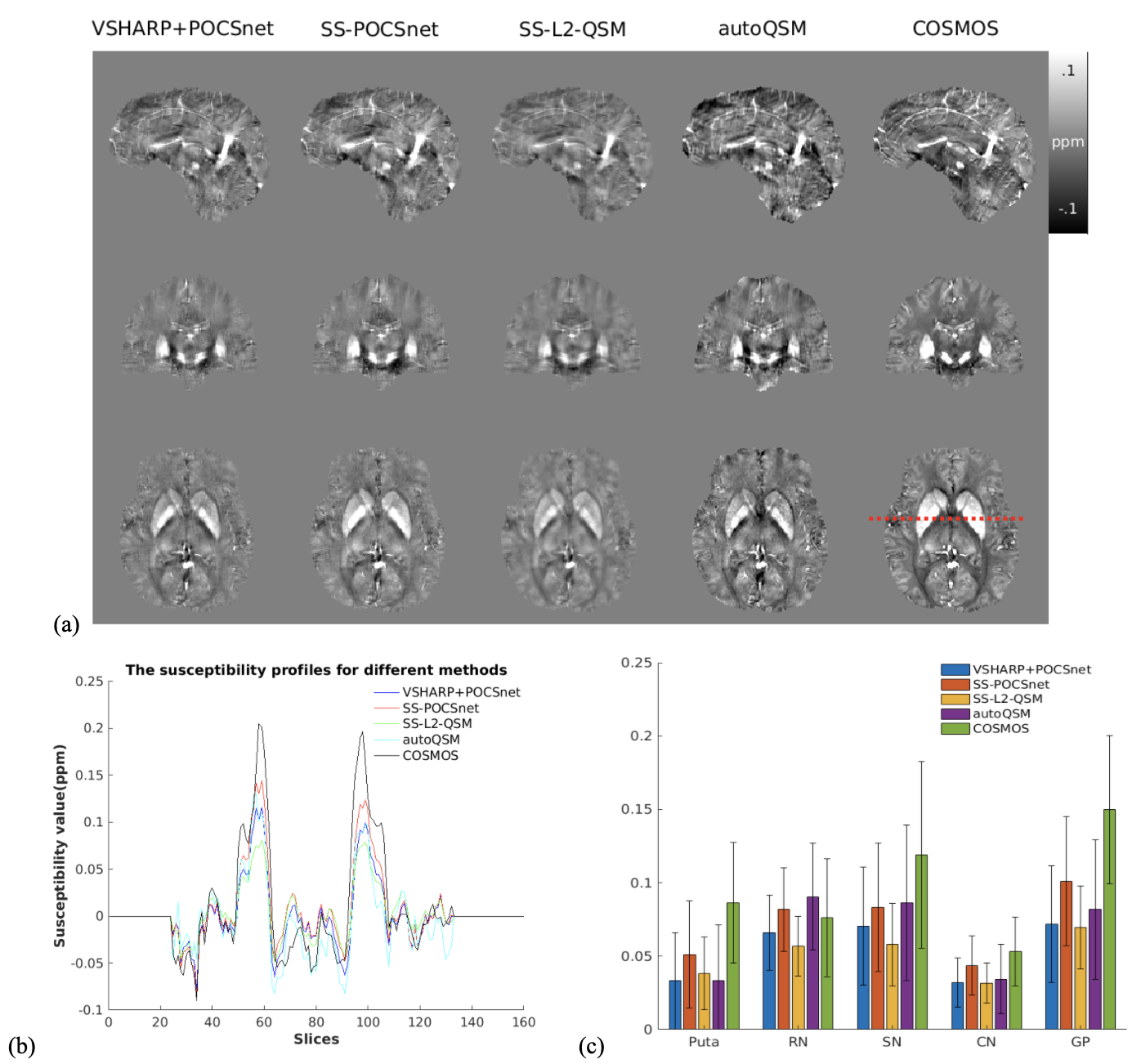
Figure 2. (a) QSM maps from VSHARP+POCSnet, SS-POCSnet, SS-L2-QSM, and autoQSM on COSMOS dataset. (b) Profiles from the location denoted by the dash line in (a). The SS-POCSnet showed higher intensities in deep brain nuclei. (c) ROI analysis in Puta, RN, SN, CN, and GP. Results from SS-POCSnet were closer to that from COSMOS compared with other methods evaluated.