4749
Investigating the dot-compartment using diffusion MRI line scanning1Centre for Advanced Imaging, University of Queensland, Brisbane, Australia, 2ARC Training Centre for Innovation in Biomedical Imaging Technology, Brisbane, Australia, 3Neuroscience Research Centre, St George's, University of London, London, United Kingdom, 4School of Mathematical Sciences, Queensland University of Technology, Brisbane, Australia
Synopsis
Diffusion MRI provides opportunities in probing tissue microstructure based on mm-scale measurements. Generally, an MRI diffusion model is used to infer biologically meaningful information from diffusion MRI measurements. Recently, there has been increasing interest in mapping the so-called dot-compartment in the human brain. The dot-compartment has been ascribed to a tissue compartment which has highly restricted diffusion. Using a custom diffusion MRI line scan we investigated the ability to obtain high b-value signals using 3T MRI equipped with 80mT/m gradients. It appears that the dot-compartment is elusive when probed using clinical standard scanners even when b-values of 15000s/mm2 are achieved.
Introduction
Diffusion MRI (dMRI) enables model based mapping of microstructural properties found in living human brain tissue,1 with a historic focus on extra- and intra-cellular diffusion2-6 and more recently slow diffusion processes.7 The challenge here is that based on the theory of mean-squared displacement, which relates displacement of water molecules in time to diffusivity, the highly restricted tissue compartment for diffusion, referred to as the dot-compartment and sometimes attributed with small spherical spaces such as cell bodies, likely has an apparent diffusion coefficient around an order of magnitude smaller than intra- and extra-cellular diffusion (~0.12µm2/ms).8 Such measurements rely on large diffusion encoding (b-value) measurements.It was shown, using the Connectome scanner with 300mT/m gradients, that there potentially exists a slowly decaying dMRI signal around b-values of 15000s/mm2 both in grey and white matter.8,9 The negative log-scale slope at large b-values provides an estimate of the apparent diffusion coefficient of the dot-compartment. Here, we investigate the presence of the dot-compartment using a 3T MRI scanner equipped with 80mT/m gradients and by using dMRI line scanning.
Methods
The study was approved by the local human research ethics committee in accordance with national guidelines. The two experienced participants were chosen in view of demonstrating low levels of motion artifact during previous MRI scans. The dMRI line scan, like a previously described approach,10 was developed by MC for use on a 3T MRI scanner (Prisma, Siemens, Erlangen, Germany). The MPRAGE scan was used as anatomical reference.MPRAGE acquisition: matrix size = 240 x 160 x 256, resolution = 1 x 1 x 1mm3, TE = 2.15ms and TR = 2500ms.
Diffusion acquisition: The dMRI line was placed perpendicular to the S1-M1 junction (see CSF6 region in Figure 1). Notably, the b-value = $$$(\gamma\delta G)^2(\Delta-\frac{\delta}{3})$$$, where $$$\gamma$$$ is the gyromagnetic ratio for hydrogen, and $$$\delta$$$, $$$\Delta$$$ and $$$G$$$ are chosen to manipulate the size of the diffusion weighting. We set $$$\delta$$$ = 20ms and $$$\Delta$$$ = 40ms and varied $$$G$$$ to achieve b-values = 5, 600, 1200, 2400, 5000, 10000, 12500 and 15000s/mm2, with TE = 75ms and TR = 2000ms. By switching on all three gradients at maximum amplitude, we were able to achieve $$$G_{max}$$$ = 138.6mT/m (i.e., $$$\sqrt{3}$$$ times 80mT/m). To control for SNR drop, the number of repetitions were set to 30 at b = 5s/mm2 and 320 by b = 15000s/mm2. Total acquisition time was around 1 hour with a 0.5 x 5 x 5mm3 line resolution.
Results and Discussion
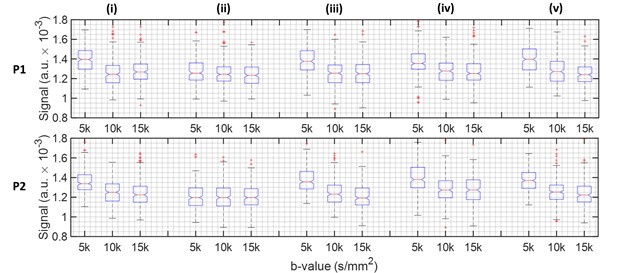
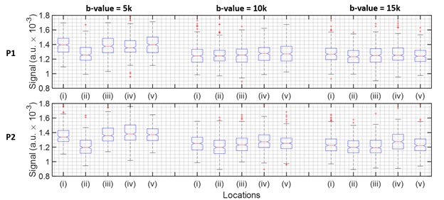
The line scan data in Figure 2 has been provided on a log-scale to be able to appreciate signal decay as a function of b-value. Figure 3 provides a zoomed in section around the S1-M1 cortical regions. Figures 4 and 5 summarise the location specific dMRI signals, particularly focusing on larger than 5000s/mm2 b-values.For the CSF region, identified as location (ii) in Figure 3, we do not expect to see any trend as a function of b-value in Figure 4, since this location has the fastest signal decay based on having the largest diffusivity. The CSF signal has decayed by b-value = 5000s/mm2, providing a baseline measure for further analysis.
At locations (i) to (v) not including (ii) as shown in Figure 3, a decaying signal trend with b-value is present and it is different at b-value = 5000s/mm2 compared with larger b-values. It is difficult to state the extent with which the dot-compartment contributes at b-values less than 10000s/mm2 because of likely partial volume effects with a 5 x 5mm2 cross-section voxel. Nonetheless, a decaying trend is likely present at location (v) in the 10000s/mm2 to 15000s/mm2 range, and appears for P2 in locations (i) and (iii). We found the log-linear negative slope in the 10000 to 15000s/mm2 range to be around an order of magnitude smaller (locations (i), (iii) and (v) for P2 in Figure 4) than ~0.12µm2/ms reported previously.8 This may be explained by a different maximum gradient strength in our study, and the differences in the protocols and b-value constituents, essentially leading to a different apparent diffusion coefficient. Considering that the observed SNR was better than expected, higher resolution (narrower line) imaging could provide a viable means to reduce partial volume effects in future work.
Conclusion
At the limit of what can be achieved using a 3T MRI scanner with 80mT/m gradients, we may have identified trends in the MRI signal at b-values larger than 10000s/mm2 that could be indicative of the presence of a dot-compartment. Further studies should explore the true signal behaviour at high b-values (i.e., linear, log-linear or power law). The interpretation of observing a linear or log-linear decay or power law behaviour would differ and may change current thought.The decreasing signal trend with b-value is in line with a previously described trend suggested to arise from the presence of a diffusion dot-compartment.8 Our observations may be strengthened by reducing the cross-sectional area of the line scan voxel, such that potential partial volume effects are reduced. Investigations into whether the dot-compartment can be observed at b-values less than 10000s/mm2 should also be explored, which may lead to spatially resolved maps of the dot-compartment volume fraction.
Acknowledgements
V. Vegh and Q. Yang were supported by an ARC discovery project grant (DP190101889). Q. Yang was also supported by an ARC DECRA fellowship grant (DE150101842). M. Cloos was supported by ARC future fellowship grant (FT200100329). The authors acknowledge the facilities and the scientific and technical assistance of the National Imaging Facility, a National Collaborative Research Infrastructure Strategy (NCRIS) capability, at the Centre for Advanced Imaging, University of Queensland.
References
1. I. Jelescu, et al, Challenges for biophysical modeling of microstructure. Journal of Neuroscience Methods, 2020, 344: 108861.
2. Y. Assaf, et al, Composite hindered and restricted model of diffusion (CHARMED) MR imaging of the human brain. NeuroImage, 2005, 27(1): 48-58.
3. Y. Assaf, et al, Axcaliber: A method for measuring axon diameter distribution from diffusion MRI. Magnetic Resonance in Medicine, 2008, 59(6): 1347-1354.
4. N. Stikov, et al, In vivo histology of the myelin g-ratio with magnetic resonance imaging. NeuroImage, 2015, 118: 397-405.
5. F. Sepehrband, et al, Brain tissue compartment density estimated using diffusion-weighted MRI yields tissue parameters consistent with histology. Human Brain Mapping, 2015, 36(9): 3687-3702.
6. Q. Yu, et al, Can anomalous diffusion models in magnetic resonance imaging be used to characterize white matter tissue microstructure? NeuroImage, 2018, 175: 122-137.
7. R. Bai, et al, Feasibility of filter-exchange imaging (FEXI) in measuring different exchange processes in human brain. NeuroImage, 2020, 219: 117039.
8. C. Tax, et al, The dot-compartment revealed? Diffusion MRI with ultra-strong gradients and spherical tensor encoding in the living human brain. NeuroImage, 2020, 210: 116534.
9. J. Veraart, et al, Noninvasive quantification of axon radii using diffusion MRI. eLife, 2020, 9: e49855.
10. M. Balasubramanian, et al, Probing in vivo cortical myeloarchitecture in human via line-scan diffusion acquisitions at 7T with 250-500 micron radial resolution. Magnetic Resonance in Medicine, 2021, 85(1): 390-403.
Figures
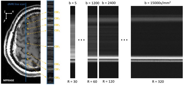
Figure 1. An example of how the dMRI line can be positioned over the brain. The CSF labels are used as landmarks in further analysis. The dMRI signals for the select b-values for the line are shown on the right over repetitions (R denotes repetitions).
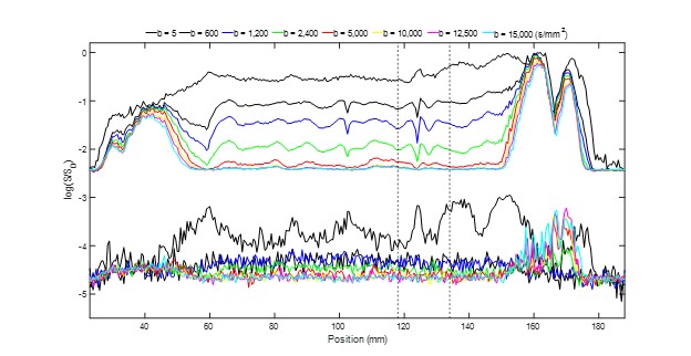
Figure 2. Illustration of dMRI line scan data for the first participant. At the top the signal averaged over repetitions is provided. The corresponding set of plots on the bottom provide the standard deviation over repetitions. Here, anterior is on the left and posterior is on the right. The large signal regions are the front and the back of the head. The dashed line identifies a region around the S1-M1 cortical junction (see Figure 3 for more detail).
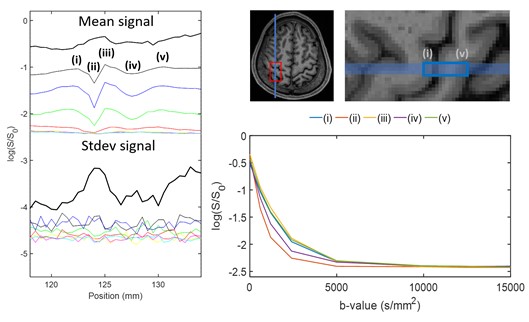
Figure 3. Illustration of the dMRI line scan around the S1-M1 region identified using the dashed lines in Figure 2. On the right anterior-posterior line positioning for the first participant is shown. Labels (i) to (v) show correspondence between the line scan and anatomical MPRAGE scan, and (ii) is the CSF region between S1 and M1. The dMRI averaged over repetitions signals are shown in the bottom right, highlighting a plateauing in the signal above a b-value of 10000s/mm2.