4699
Implementation of the QRAPMASTER sequence using a dictionary matching and quantitative evaluation of the magnetization transfer effect
Katsumi Kose1, Ryoichi Kose1, and Yasuhiko Terada2
1MRIsimulations Inc., Tokyo, Japan, 2University of Tsukuba, Tsukuba, Japan
1MRIsimulations Inc., Tokyo, Japan, 2University of Tsukuba, Tsukuba, Japan
Synopsis
The magnetization transfer effect of the QRAPMASTER sequence was investigated using phantom experiments and Bloch simulations. The phantom consisted of MnCl2 aqueous solution with various proton T1 values and raw chicken breast meat. T1 values of the MnCl2 solution measured using the QRAPMASTER sequence showed excellent linear relation with those measured with the standard method. However, T1 of the chicken breast sample deviated far from the linear regression line. The results suggested that the T1 values of biological samples measured by the QRAPMASTER sequence are underestimated compared to those measured by the standard method.
Introduction
Recent studies report importance of the magnetization transfer (MT) effect [1-2] on quantitative magnetic resonance imaging [3-10]. Although many studies have been reported on the MT effect in multislice imaging [11-14], to the best of our knowledge, the MT effect on the QRAPMASTER sequence [15] has not yet been reported.Materials and methods
The phantom consisted of seven test tubes (16mm OD; 14mm ID). Six test tubes were filled with MnCl2 aqueous solution (T1 ~ 500-1000 ms). One test tube was filled with raw chicken breast meat. The phantom was imaged with a small horizontal-bore 1.5 T MRI system [16]. Pulse sequences were multislice multiple spin-echo (MSMSE) and QRAPMASTER sequences. The QRAPMASTER sequence was developed by inserting saturation pulses (FA=120°, SLR design) into the sequential-order MSMSE sequence. The sequence parameters were; number of slices = 11, slice thickness = 5 mm, slice gap = 0 mm, FOV = (64 mm)2, image matrix = 2562, TR = 2200 ms. The number of echoes and echo spacing of the MSMSE were 8 and 12 ms. Effective TE of the QRAPMASTER sequence was 12 and 60 ms. The shape of the 90° and 180° pulses was a hamming-windowed sinc with seven side lobes. The duration times of the RF pulses were both 1 ms and the theoretical peak intensities were 47.083 and 94.166 μT. The excitation frequency varied from -40 to +40 in 8 kHz steps. The delay time (TD) for the QRAPMASTER sequence varied from 420 to1420 in 200 ms steps. Relaxation times of the phantom were calculated using a data matching between the series of image datasets experimentally acquired and dictionary datasets calculated by Bloch simulations. The Bloch image simulations were performed using a Bloch simulator (BlochSolver) [16]. The MT effect was evaluated by numerically solving modified Bloch equations for a two-pool model [17].Results
Figs.1(a)-(c) show the first-echo real-part images of the central section acquired with the single-slice multiple SE, interleave MSMSE, and sequential MSMSE sequences. Figs.1(d)-(f) are the difference images of Figs.1(a)-(c). The image intensity ratio of the chicken breast sample shown in Figs.1(a)-(c) was 1:0.82:0.73. Figs.2(a)-(c) show the first-echo real-part images of the central section simulated with the same sequences as shown in Figs.1(a)-(c). The calculation time for one MSMSE image were about 4 hours using 91,750,240 isochromats and RTX2080Ti GPU. Gaussian noise of the same level as experiments was added on the simulated images. The image intensity difference between the multislice and the single-slice images was not observed for the central sample because the MT effect was not incorporated in the Bloch image simulation. Fig.3 shows the absolute value first-echo images of the central section acquired by the QRAPMASTER sequence at TD = 420-1620 ms.Fig.4(a) shows the T1 maps obtained by the QRAPMASTER sequences. Fig.4(b) shows the T1 values averaged over the ROI in the T1 maps plotted against those measured by the standard method. Blue and orange dots indicate the T1 values of the MnCl2 solution and the chicken breast sample. Fig.4(c) shows the T2 maps obtained by the MSMSE sequence. Fig.4(d) shows the T2 values averaged over the ROI in the T2 maps plotted against those measured by the standard method. Blue and orange dots indicate the T2 values of the MnCl2 solution and the chicken breast sample.
Figs.5(a)-(b) show the temporal variation of Mz of the chicken breast sample (sample 7) calculated for the central slice with the MSMSE sequences with and without the MT effect. Fig.5(c) shows the temporal variations of Mz of sample 7 calculated with the single-slice and sequential MSMSE sequences. The image intensity ratio of sample 7 shown in Figs.5(a)-(c) was 1:0.73:0.67. Figs.5(d)-(e) show the temporal variation of Mz of sample 7 calculated for the central slice with the QRAPMASTER sequences. The points on the graphs represent Mz just before the 90° pulses for each slice. Fig.5(f) shows Mz with and without the MT effect plotted against TD. These curves were fitted to exponential functions with single time constants of 929 ms and 1021 ms. Figs.5(g)-(h) show the temporal variation of Mz of sample 7 calculated for the central slice with the QRAPMASTER sequences having 3.2 times pulse width. The FA of the refocusing pulse was 180°. Fig.5(i) shows Mz with and without MT effects plotted against TD. The recovery curves were fitted to exponential functions with single time constants of 862, 810, and 702 ms for 90°, 120°, and 180° flip angles of the refocusing pulses, and 1024 ms calculated without the MT effect.
Discussion
T1 values of the chicken breast samples were far from the regression lines of T1 of MnCl2 solution measured by the QRAPMASTER sequence. The T1 shortening of the chicken breast sample was semi-quantitatively explained by the Bloch simulation for the two-pool model. The difference between the observed value (~750 ms) and calculated value (~930 ms) may be due to the theoretical absorption line shape (super-Lorentzian) of the sample, assumed two-pool model parameters, and neglection of the slice width effect. In conclusion, this study suggested that the MT effect shortens the T1 values of biological samples obtained by the QRAPMASTER sequence.Acknowledgements
No acknowledgement found.References
[1] Wolff SD, Balaban RS. Magnetization transfer contrast (MTC) and tissue water proton relaxation in vivo. Magn. Reson. Med. 1989;10:135–144. [2] Henkelman RM, Huang X, Xiang QS, Stanisz GJ, Swanson SD, Bronskill MJ. Quantitative interpretation of magnetization transfer. Magn Reson Med. 1993;29:759-66. [3] Wood TC, Malik SJ. Magnetization Transfer. In: Seiberlich N, Gulani V, editors. Quantitative Magnetic Resonance Imaging, Elsevier; 2020, p. 839-856. [4] Ou X, Gochberg DF. MT effects and T1 quantification in single-slice spoiled gradient echo imaging. Magn Reson Med. 2008;59:835-45. [5] Crooijmans HJ, Gloor M, Bieri O, Scheffler K. Influence of MT effects on T2 quantification with 3D balanced steady-state free precession imaging. Magn Reson Med. 2011;65:195-201. [6] van Gelderen P, Jiang X, Duyn JH. Effects of magnetization transfer on T1 contrast in human brain white matter. Neuroimage. 2016;128:85-95. [7] Liu F, Block WF, Kijowski R, Samsonov A. Rapid multicomponent relaxometry in steady state with correction of magnetization transfer effects. Magn Reson Med. 2016;75:1423-33. [8] Radunsky, D, Blumenfeld-Katzir, T, Volovyk, O, Tal, A, Barazany, D, Tsarfaty, G, Ben-Eliezer, N. Analysis of magnetization transfer (MT) influence on quantitative mapping of T2 relaxation time. Magn Reson Med. 2019;82:145–158. [9] Teixeira RPAG , Malik SJ , Hajnal JV . Fast quantitative MRI using controlled saturation magnetization transfer. Magn Reson Med. 2019;81:907-920. [10] Teixeira RPAG, Neji R, Wood TC, Baburamani AA, Malik SJ, Hajnal JV. Controlled saturation magnetization transfer for reproducible multivendor variable flip angle T1 and T2 mapping. Magn Reson Med. 2020 84:221-236. [11] Dixon WT, Engels H, Castillo M, Sardashti M. Incidental magnetization transfer contrast in standard multislice imaging. Magn Reson Imaging 1990;8:417–422. [12] Melki PS, Mulkern RV. Magnetization transfer effects in multislice RARE sequences. Magn Reson Med 1992;24:189–195. [13] Santyr GE. Magnetization transfer effects in multislice MR imaging. Magn Reson Imaging 1993;11:521–532. [14] Weigel M, Helms G, Hennig J. Investigation and modeling of magnetization transfer effects in two-dimensional multislice turbo spin echo sequences with low constant or variable flip angles at 3 T. Magn Reson Med. 2010;63:230-4. [15] Warntjes JBM, Leinhard OD, West J, Lundberg P. Rapid magnetic resonance quantification on the brain: optimization for clinical usage. Magn Reson Med 2008;60:320–9. [16] Kose R, Kose K. BlochSolver: a GPU-optimized fast 3D MRI simulator for experimentally compatible pulse sequences. J Magn Reson 2017;281:51–65. [17] Graham SJ, Henkelman RM. Understanding pulsed magnetization transfer. J Magn Reson Imaging. 1997;7:903-912.Figures
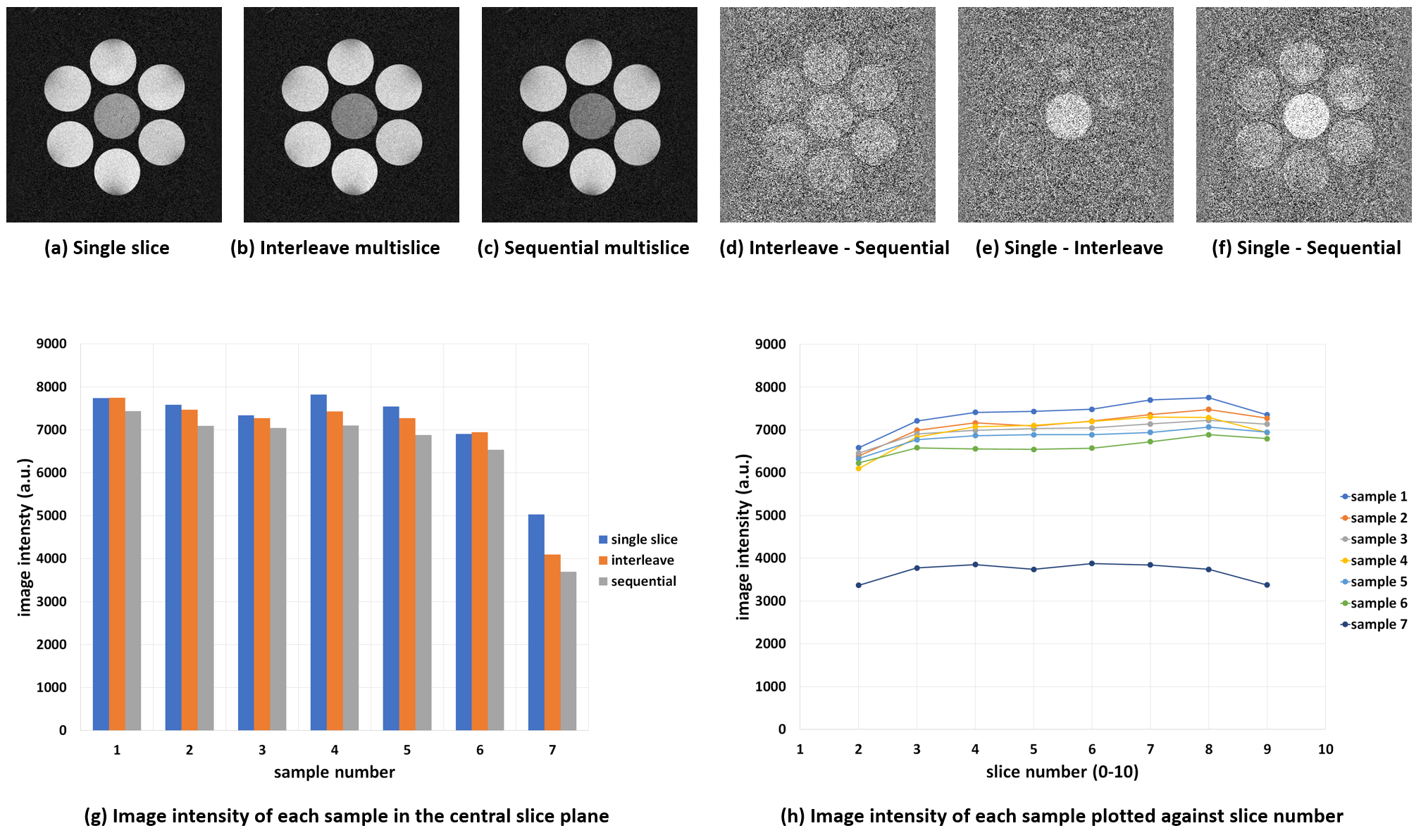
The central cross-sections experimentally acquired
with the single slice (a), interleave multislice (b), and sequential multislice
(c) pulse sequences. (d)-(f) show the difference images between (b) and
(c), (a) and (b), and (a) and (c), respectively. All images were real part
images obtained after phase correction. (g) Image intensities averaged over
small circular areas in each sample of the three cross-sectional images shown
in (a)-(c). (h) Image intensity of each sample
plotted along the slice direction. 8 slices out of 11 slices are plotted.
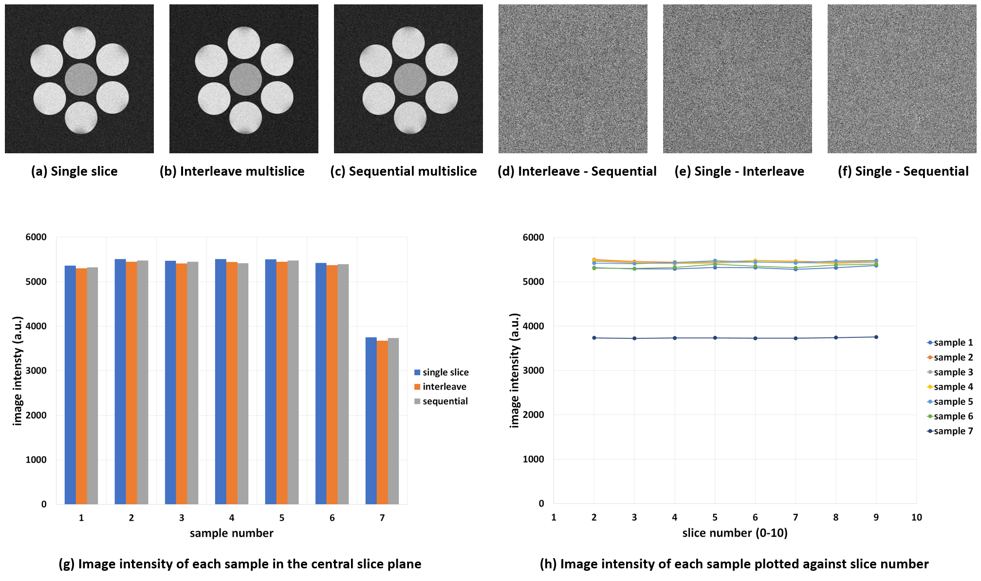
The central cross-sections simulated for the
single slice (a), interleave multislice (b), and sequential multislice (c) sequences
using the Bloch simulator. Gaussian noise is artificially superimposed over the
images. (d)-(f) show the difference images between (b) and
(c), (a) and (b), and (a) and (c), respectively. All images were real part
images. (g) Image intensities averaged over small circular areas in each sample
for the three cross-sectional images shown in (a)-(c). (h) Image intensity of each sample
plotted along the slice direction.
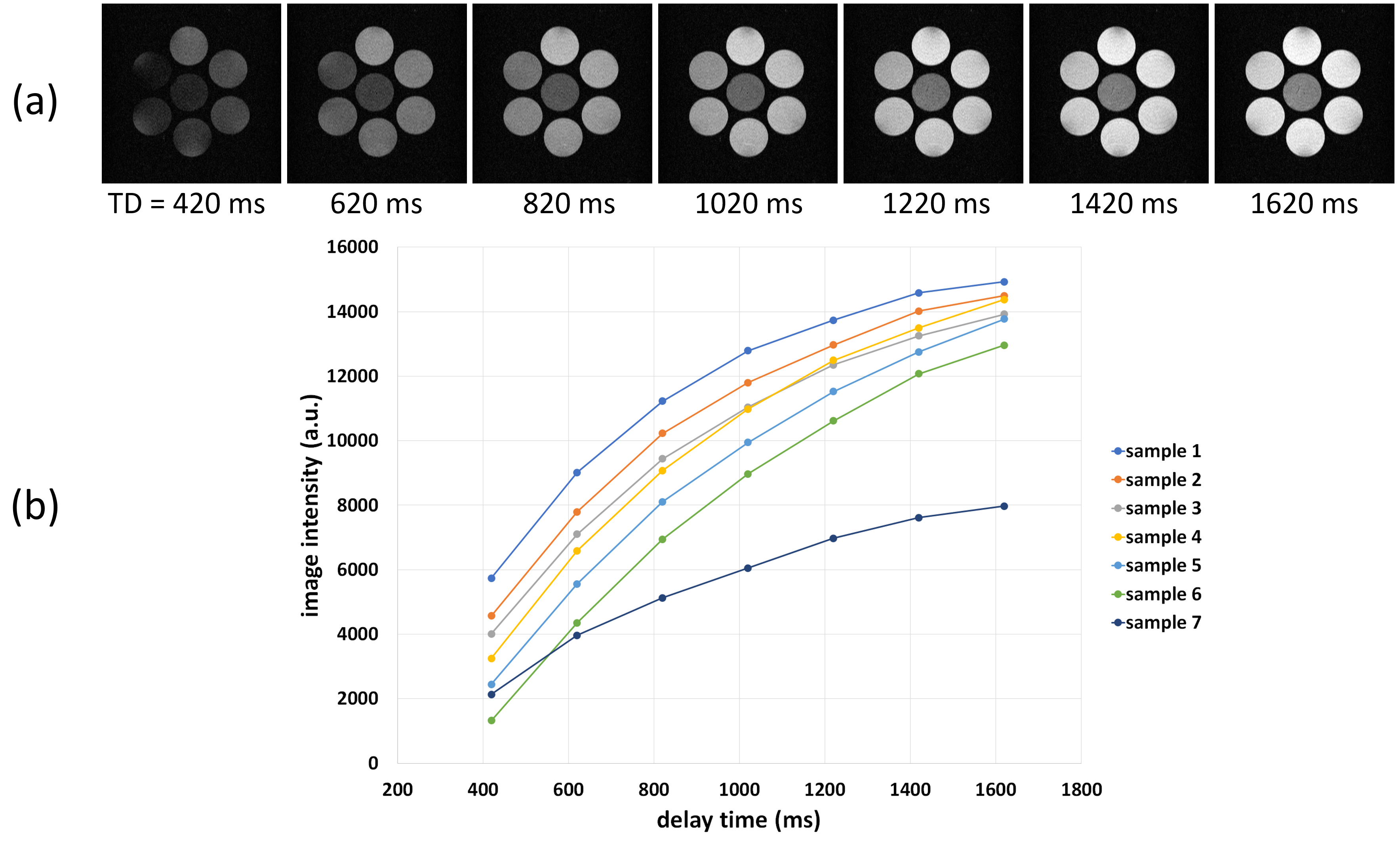
(a) Magnitude images of the central cross-section
acquired with the QRAPMASTER sequences. (b) Image intensity of the magnitude
images plotted against the delay time.
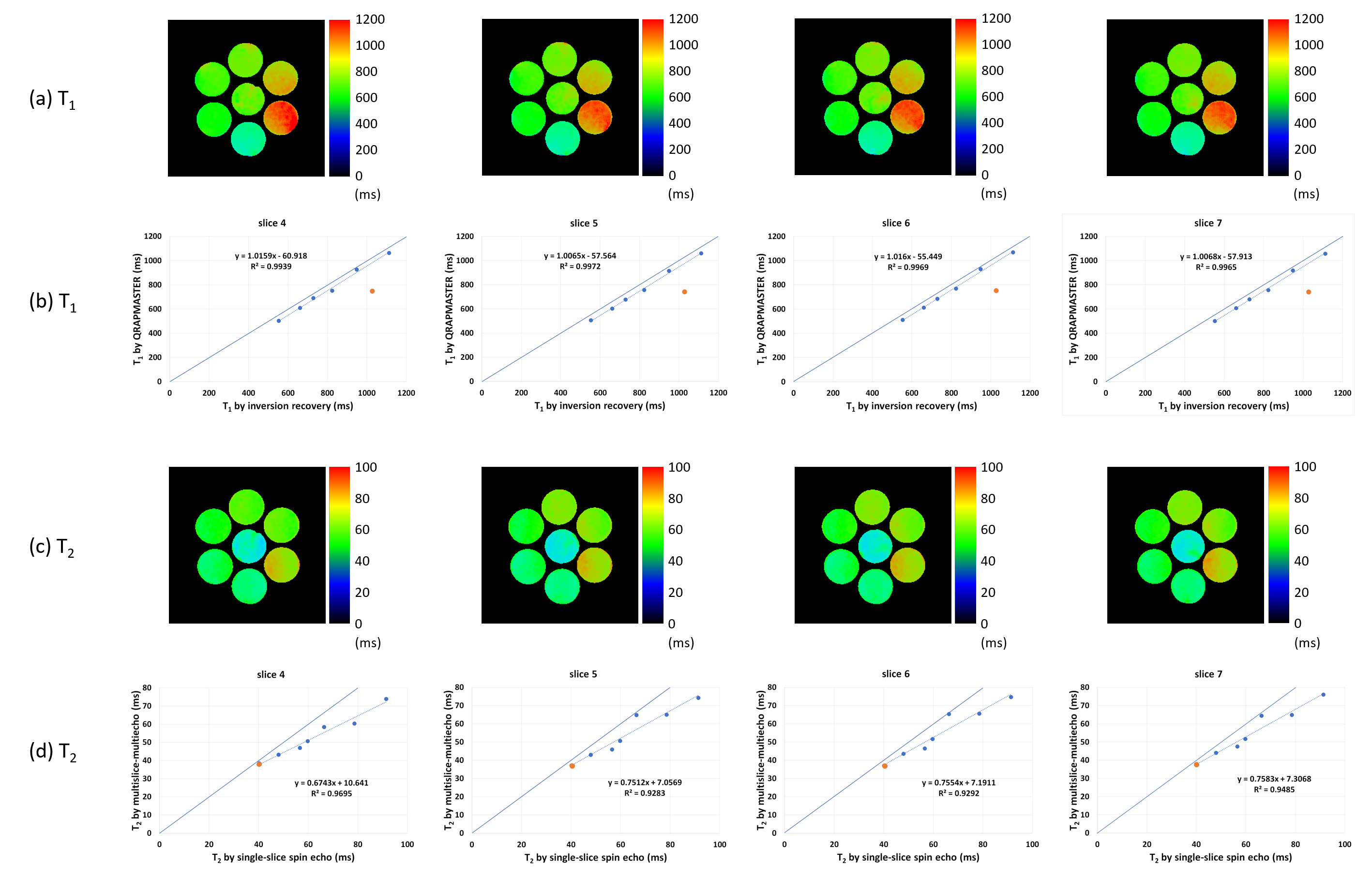
(a) T1 maps of four consecutive
slices calculated from the QRAPMASTER sequence. (b) Scatter plots of the T1
values. The calculated T1 values are plotted against those measured
by the standard method. The blue and orange points show T1 for the MnCl2
solution and the chicken breast sample. (c) T2 maps of the four
consecutive slice planes calculated from the sequential MSMSE sequence. (d) Scatter
plots of the T2 values. The calculated T2 values are
plotted against those measured by the standard method. The blue and orange
points show T2 values for the MnCl2 solution and the
chicken sample.
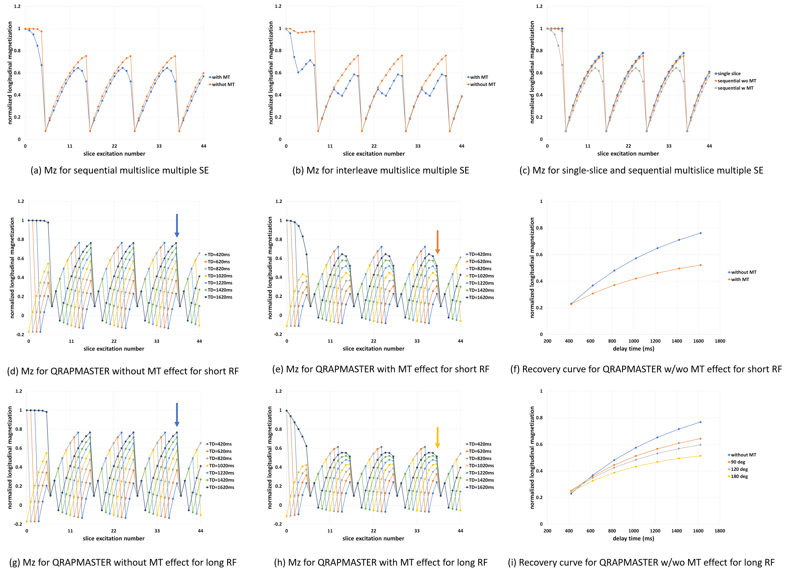
(a)-(b) Mz of the sample 7 (chicken breast) calculated
with the sequential (a) and interleave (b) MSMSE with and without MT. (c) Mz of
the sample 7 calculated with the single slice sequence. (d)-(e) Mz of the sample 7 calculated with the
QRAPMASTER without (d) and with (e) MT. The RF pulse width was 1.0 ms (f) Mz of
the sample 7 with and without MT plotted against TD. (g)-(h) Mz of the sample 7 calculated with the
QRAPMASTER without (g) and with (h) MT. The RF pulse width was 3.2 ms and the FA
of the refocusing pulses was 180°. (i) The Mz of the sample 7 with and without (blue)
MT plotted against TD.
DOI: https://doi.org/10.58530/2022/4699