Introduction

To reconstruct high-quality images from sparsely sampled k-space data, SENSE-based parallel imaging methods require good coil sensitivity functions^1-7. A common approach to sensitivity estimation is to acquire auto-calibration data that fully sample central k-space^2,4,7,8. Yet, inaccurate sensitivity estimation from limited auto-calibration data may lead to reconstruction artifacts, especially when the acceleration factor is large. To improve the accuracy of coil sensitivity estimation, joint estimation and reconstruction techniques (e.g., JSENSE) have been proposed, which use all the measured data to iteratively estimate coil sensitivity functions and the images^4,9.

This paper presents a new method for joint estimation of coil sensitivity functions and image reconstruction from sparsely sampled k-space data. The proposed method uses a probabilistic subspace model to capture statistical spatial distributions of a given coil from past scans, which makes it possible to eliminate the acquisition of auto-calibration data. Calibationless scans allow higher acceleration factors, permit flexible k-space trajectories, and are immune to motion-induced mismatches¹⁰. We have validated the proposed method using publicly available fastMRI dataset¹¹, producing high-quality reconstructions from calibrationless sparse data.

Method

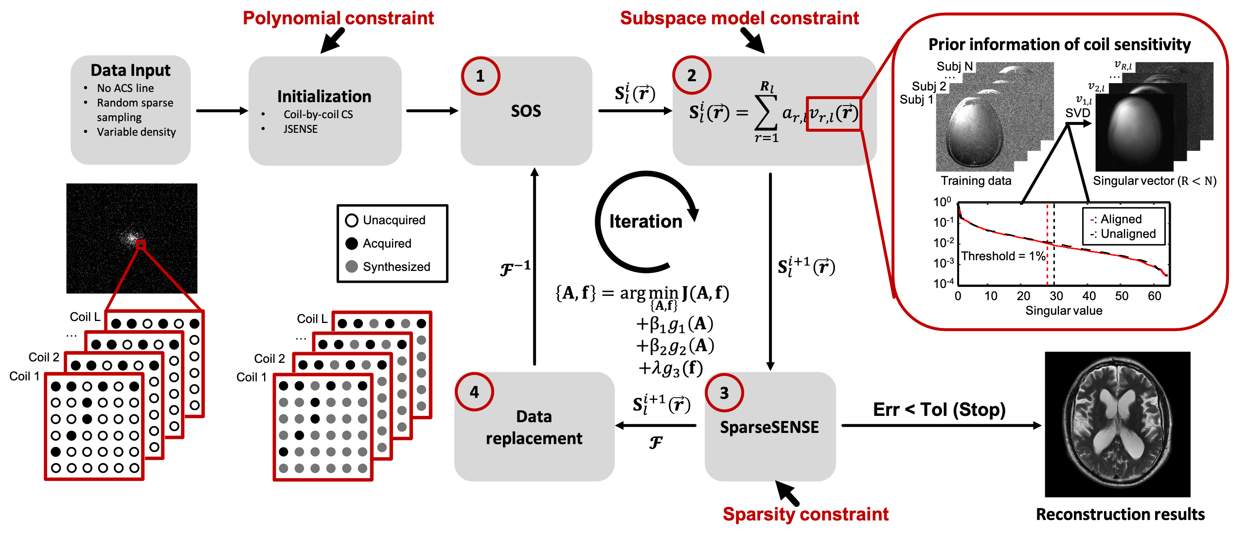
The proposed method has a couple of key features: a) using a probabilistic subspace model to capture the statistical spatial distributions of a given coil from training data acquired under different conditions, and b) exploiting correlation among different coils to improve the estimation of the coil sensitivity functions.

To construct the probabilistic subspace model, we rearranged the $$$l^{th}$$$ coil’s data $$$\left\{S^{(n)}_l(\mathbf{r})\right\}^N_{n=1}$$$ into the following Casorati matrix after aligning the training data using ANTs¹²:$$C_{l}=\left[\begin{matrix}S^{(1)}_l(\mathbf{r}_1)&S^{(1)}_l(\mathbf{r}_2)&\dots&S^{(1)}_l(\mathbf{r}_M)\\S^{(2)}_l(\mathbf{r}_1)&S^{(2)}_l(\mathbf{r}_2)&\dots&S^{(2)}_l(\mathbf{r}_M)\\\vdots&\vdots&\ddots&\vdots\\S^{(N)}_l(\mathbf{r}_1)&S^{(N)}_l(\mathbf{r}_2)&\dots&S^{(N)}_l(\mathbf{r}_M)\end{matrix}\right]\tag{1}$$and applied singular value decomposition (SVD) to $$$C_l$$$. We chose the $$$R_l$$$ principal right-singular vectors $$$\left\{v_{r,l}(\mathbf{r})\right\}^{R_l}_{r=1}$$$ as the coil sensitivity basis functions and expressed the desired sensitivity function as a linear combination of pre-learned basis functions: $$$S_l(\mathbf{r})={\textstyle\sum_{r=1}^{R_l}a_{r,l}v_{r,l}(\mathbf{r})}$$$. We further treated $$$\left \{a_{r,l}\right\}^{R_l}_{r=1}$$$ as random variables and use their distributions $$$P\left (\left\{a_{r,l}\right\}\right )$$$ to capture the statistical distributions of the sensitivity function of a given coil under different scan conditions. For simplicity, we approximated the distribution $$$P\left (\left\{a_{r,l}\right\}\right )$$$ as a Gaussian function $$$N(u_{r,l},\sigma^2_{r,l})$$$ and estimated it from the training data. This probabilistic subspace representation imposes strong statistical spatial prior information on the sensitivity functions, which helps estimate sensitivity functions from highly sparse data.

To exploit the correlation among different coils, the following Casorati matrix of a given data set was forced to be low-rank by minimizing its nuclear norms:$$C=\left[\begin{matrix}S_1(\mathbf{r}_1)&S_1(\mathbf{r}_2)&\dots&S_1(\mathbf{r}_M)\\S_2(\mathbf{r}_1)&S_2(\mathbf{r}_2)&\dots&S_2(\mathbf{r}_M)\\\vdots&\vdots&\ddots&\vdots \\S_L(\mathbf{r}_1)&S_L(\mathbf{r}_2)&\dots&S_L(\mathbf{r}_M)\end{matrix}\right].\tag{2}$$
These constraints were integrated using an iterative algorithm (Figure 1). For initialization, we performed coil-by-coil compressed sensing (CS) reconstruction with coil correlation constraint and JSENSE. We then iteratively updated both the coefficients of sensitivity functions $$$\mathbf{A}$$$ and the desired image $$$\mathbf{f}$$$ with the following steps:

Step 1: Sensitivity estimation:$$S_l(\mathbf{r})=\frac{\hat{f_l}(\mathbf{r})}{\sqrt{{\textstyle\sum_{l=1}^{L}\left|\hat{f_l}(\mathbf{r})\right|}^2}},\tag{3}$$ where $$$\hat{f_l}(\mathbf{r})$$$ is reconstructed individual-coil image. Then we aligned $$$S_l(\mathbf{r})$$$ and the pre-learned subspace.

Step 2: Sensitivity coefficients estimation:$$arg \min_{\left\{\mathbf{A}_l\right\}^L_{l=1}}\sum_{l=1}^{L}\left\|\mathbf{S}_l-\mathbf{A}_l\mathbf{V}_l\right\|^2_2-\beta_1logP(\left\{\mathbf{A}_l\right\})+\beta_2\left\|C\right\|_*,C=\left[\mathbf{A}_1\mathbf{V}_1|\dots|\mathbf{A}_L\mathbf{V}_L\right]^T.\tag{4}$$ Probability distribution and coil correlation constraints were employed in this step to improve the accuracy of coefficients estimation.

Step 3: SparseSENSE reconstruction:$$\mathbf{f}=arg\min_{\mathbf{f}}\sum_{l=1}^{L}\left\|\mathbf{d}_l- \mathbf{\Omega FS}_l\left\{\mathbf{f}\right\}\right \|^2_2+\lambda\left\|\Psi\left(\mathbf{f}\right)\right\|_1,\tag{5}$$ where $$$\mathbf{\Omega}$$$, $$$\mathbf{f}$$$, and $$$\mathbf{S}_l$$$ are the operators accounting for sampling, Fourier encoding, and the coil sensitivity function of the $$$l^{th}$$$ coil estimated from step 2, respectively; $$$\mathbf{d}_l$$$ is the vector of undersampled measured k-space data of the $$$l^{th}$$$ coil; $$$\mathbf{\Psi}$$$ donates wavelet transform.

Step 4: Data replacement to impose data consistency.

These steps were repeated until the errors of estimated sensitivity function $$$\mathbf{S}_l$$$ and image $$$\mathbf{f}$$$ of two iterations were smaller than a chosen toleration level.

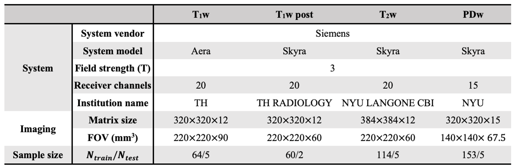
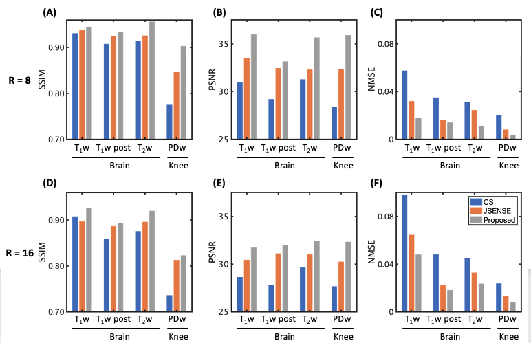
Evaluation was performed on the fastMRI dataset¹¹. Training data and test data were collected from the same scanner using the same receiver system (Table 1). The brain and knee images were retrospectively undersampled in k-space in a variable-density pattern (R=8,16). We tested our image reconstruction algorithm in T₁w, T₁w post, T₂w brain images, and PDw knee images. Coil-by-coil CS and JSENSE with polynomial model were performed for comparisons^4,13. Structural similarity (SSIM) index, peak signal to noise ratio (PSNR), and normalized mean squared error (NMSE) were also used to assess the reconstructions obtained using the proposed method in comparison with CS and JSENSE.

Results and Discussion

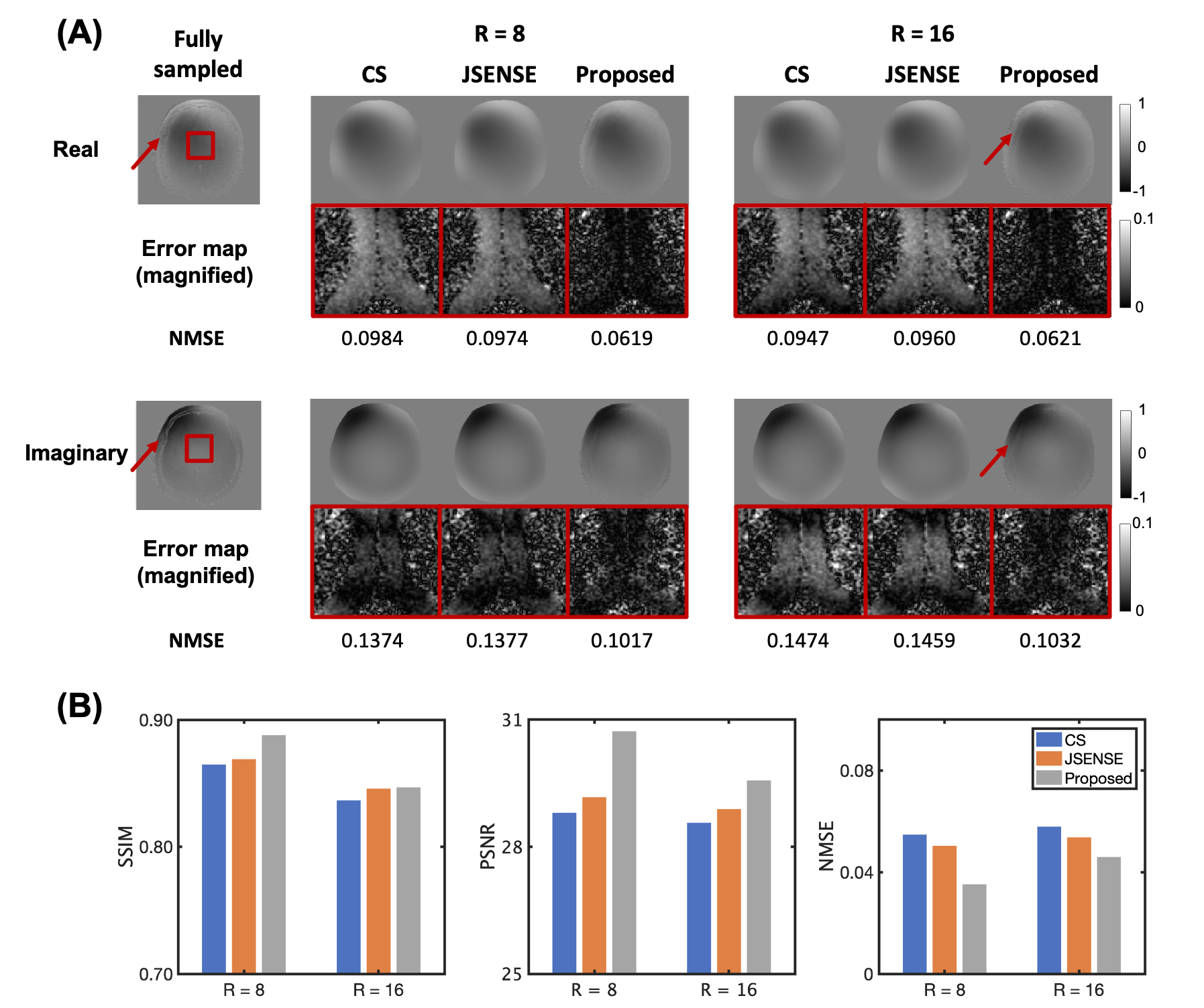
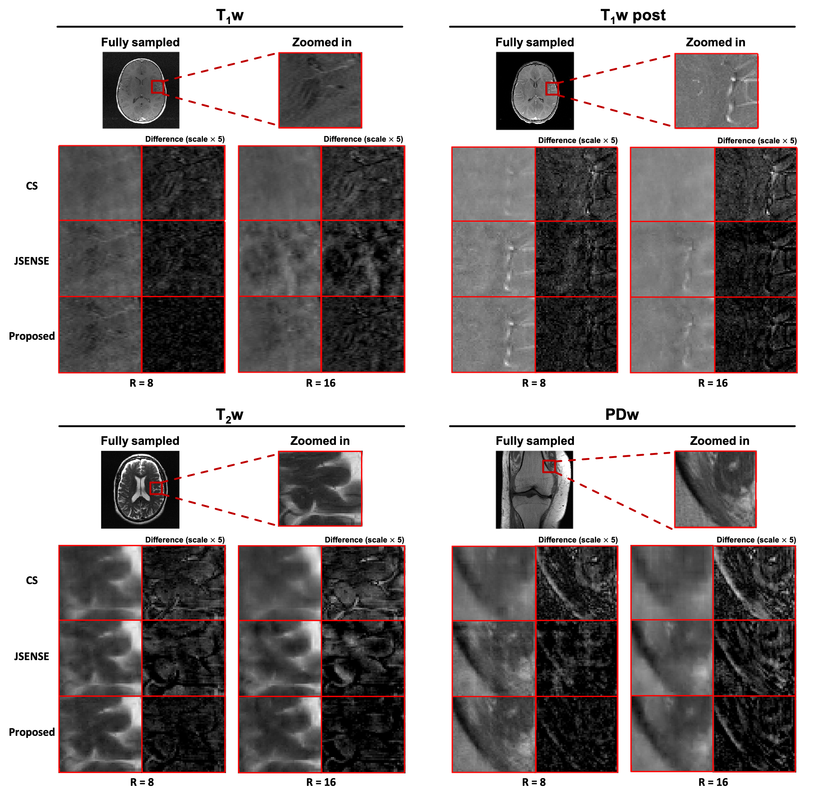
Representative coil sensitivity functions estimated from highly accelerated (R=8,16) calibrationless data are shown in Figure 2A. Compared to the ground truth, the proposed method recovered the fine details between the brain tissue and CSF as well as skull edge well, which were lost in the CS and JSENSE reconstructions. The proposed method also resulted in better image quality than the corresponding SENSE reconstruction (Figure 2B).

As can be seen from Figures 3 and 4, the proposed reconstructions scored the highest SSIM, highest PSNR, and lowest NMSE for all the images tested. Specifically, for the T₂w and PDw images with sharp image contrast and larger training dataset, the reconstructions seem to benefit even more from the proposed method.

Conclusions

This work presents a new method for joint estimation of coil sensitivity functions and image reconstruction from sparsely sampled calibrationless k-space data, using a probabilistic subspace model to capture the statistical spatial distributions of a given coil from prior scans. The proposed method has been validated by experimental data, producing high-quality reconstruction results. With further improvement, the method may further enhance the practical utility of parallel imaging.

Acknowledgements

N/A