4496
Magnetic Resonance Spectroscopy Frequency and Phase Correction Using Convolutional Neural Networks1Department of Biomedical Engineering, Columbia University, New York, NY, United States, 2Department of Psychiatry, Columbia University, New York, NY, United States, 3Radiology and Biomedical Imaging of Biomedical Engineering, Yale University, New Haven, CT, United States, 4Department of Neurology, Columbia University, New York, NY, United States, 5Taub Institute Research on Alzheimer's Disease and the Aging Brain, Columbia University, New York, NY, United States, 6Mortimer B. Zuckerman Mind Brain Behavior Institute, Columbia University, New York, NY, United States
Synopsis
Frequency and Phase Correction (FPC) is an essential technique to resolve frequency and phase shifts that arise in Magnetic Resonance Spectroscopy (MRS). As of today, a deep learning method using multilayer perceptrons has been developed to correct these shifts. However, a more robust network such as convolutional neural networks (CNN) can be considered as this approach more accurately obtains spatial information and extract key features of the given data. In this study, we aim to investigate the feasibility and utility of CNNs for FPC of single voxel MEGA-PRESS MRS simulated and in vivo data.
Introduction
Magnetic Resonance Spectroscopy (MRS) is a widely available approach for research and for routine clinical applications. However MR is highly sensitive to scanner instabilities such as frequency drift and subject motion, which can result in frequency and phase shifts that affect data analysis1,2. Thus, frequency-and-phase correction (FPC) is an important technique that needs to be performed. Deep learning is an effective image processing approach that has been adopted in MR imaging and a multilayer perceptron (MLP) model has been recently applied to single-transient FPC for edited MRS3. Although MLP provides quick and yields well-predicted results, a more robust network could be considered, such as a convolutional neural network (CNN) to more accurately obtain spatial information and extract key features of the input data for FPC. In the present study, we aim to investigate the feasibility and utility of CNNs for FPC of single voxel MEGA-PRESS MRS simulated and in vivo data.Material and Methods
2.1 Simulated DatasetThe MEGA-PRESS transients were simulated using the FID-A toolbox1,4,5. The training set for the CNN model was allocated 36,000 OFF+ON spectra, the validation set was allocated 4,000, and the test set was allocated 1000. Furthermore, additional spectra were created with lower SNRs (10, 5, and 2.5) by adding random Gaussian noise to the published simulated dataset respectively.
2.2 In vivo Dataset
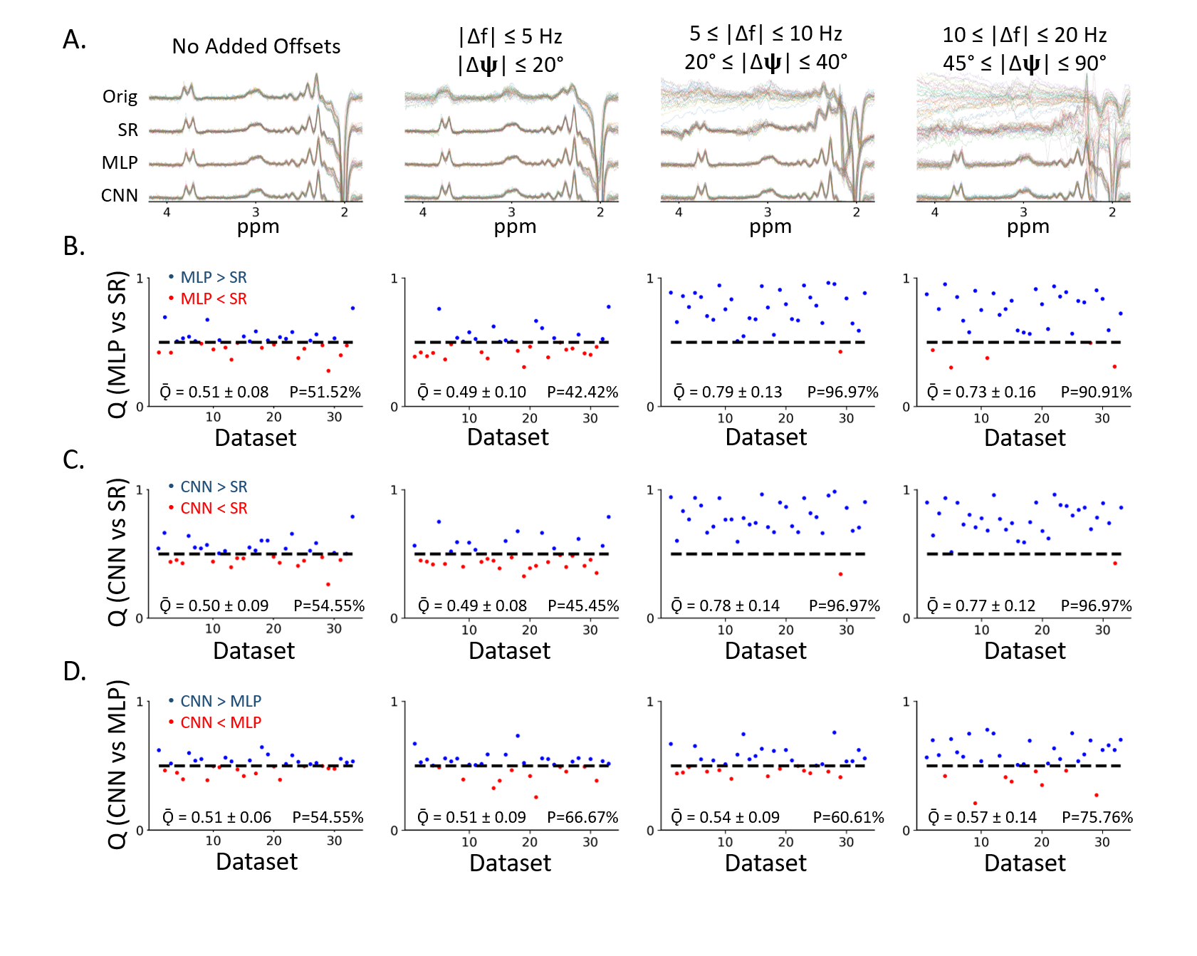
Thirty-three MEGA-edited datasets (320 transients OFF+ON each) were retrieved from the publicly available Big GABA repository and tested on our CNN model1. Additional offsets (C1: 0≤|∆f|≤5 Hz and 0°≤|∆φ|≤20°; C2: 5≤|∆f|≤10 Hz and 20°≤|∆φ|≤45°; C3: 10≤|∆f|≤20 Hz and 45°≤|∆φ|≤90°) were also applied to the in vivo dataset to evaluate the performance.
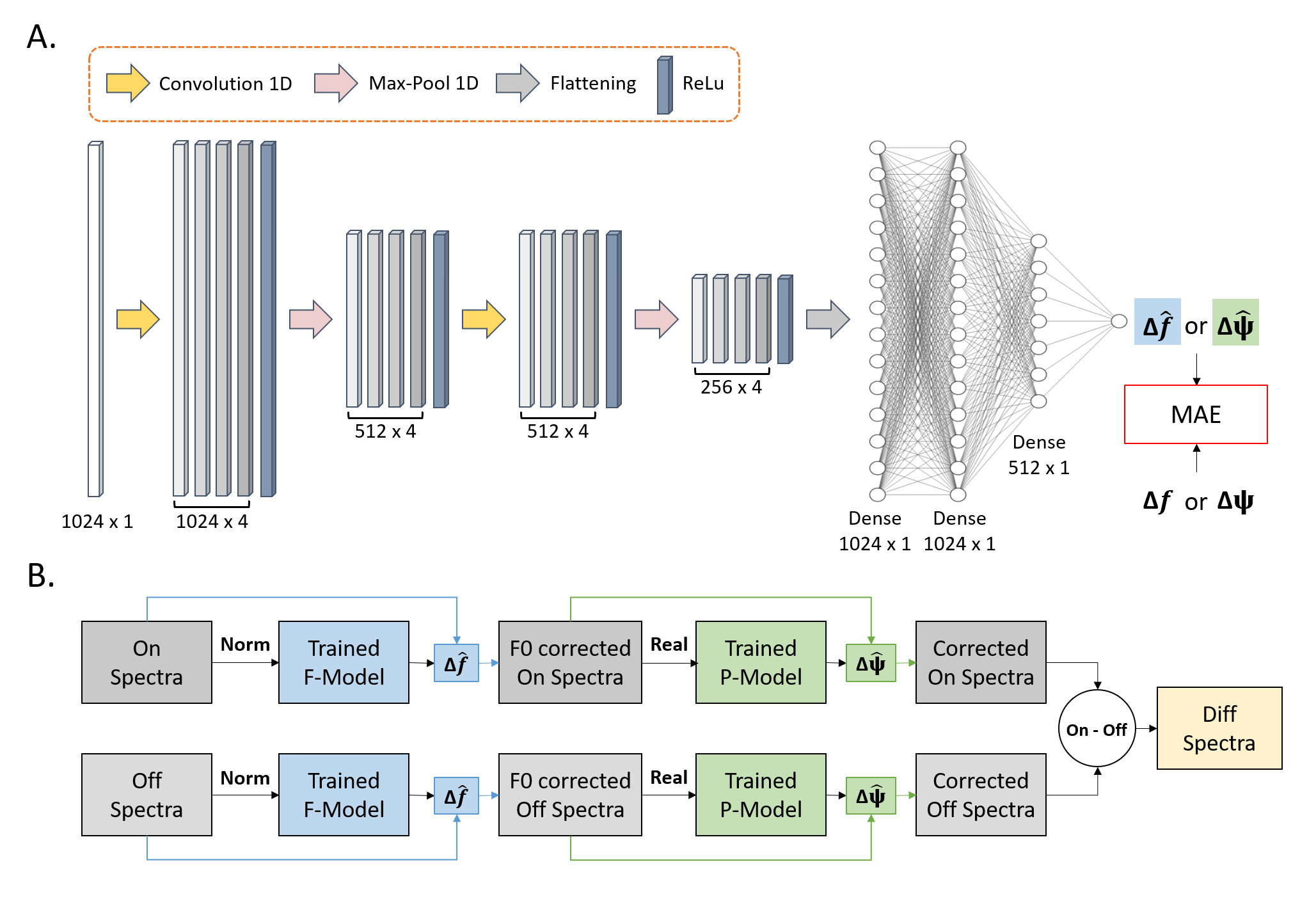
2.3 Network architecture
A CNN model was evaluated by computing the accuracy in frequency and phase offset prediction (Figure 1A). The CNN model was implemented as sequential networks (F-model and P-model) and the same architecture (Figure 1B) was used for both models. The magnitude spectrum was used as input for the F-model and the real spectrum was used as input for the P-model. An Adam optimizer was used to train the neural network with a 0.01 learning rate6. Each model was trained for 300 epochs with a batch size of 32, and the mean absolute error was used as the loss function.
2.4 Performance Measurement
In the simulated dataset, the artificial offsets were set as the ground truth, and the mean absolute error between the ground truth and predicted value was used as the criteria to measure the network's performance. For the in vivo dataset, a P and Q score was used to determine the performance strengths of each method1.
Results
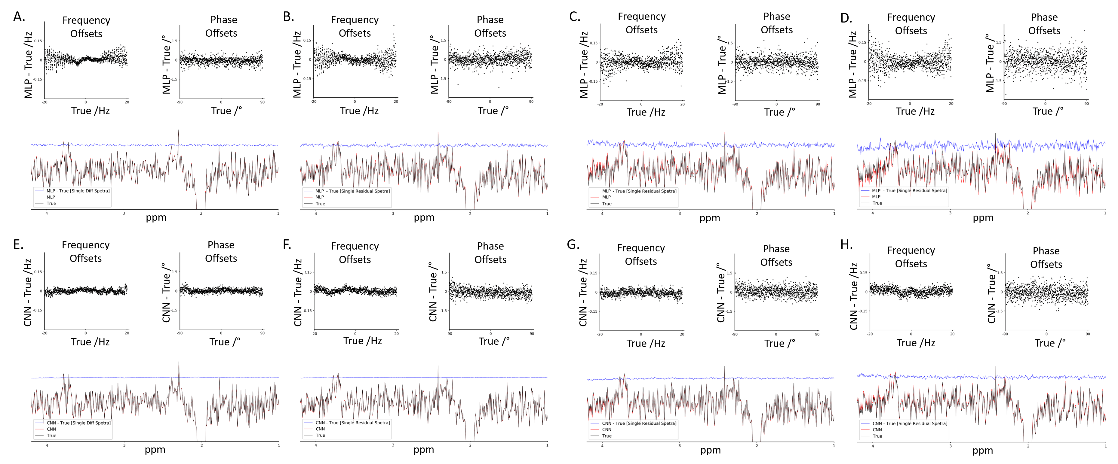
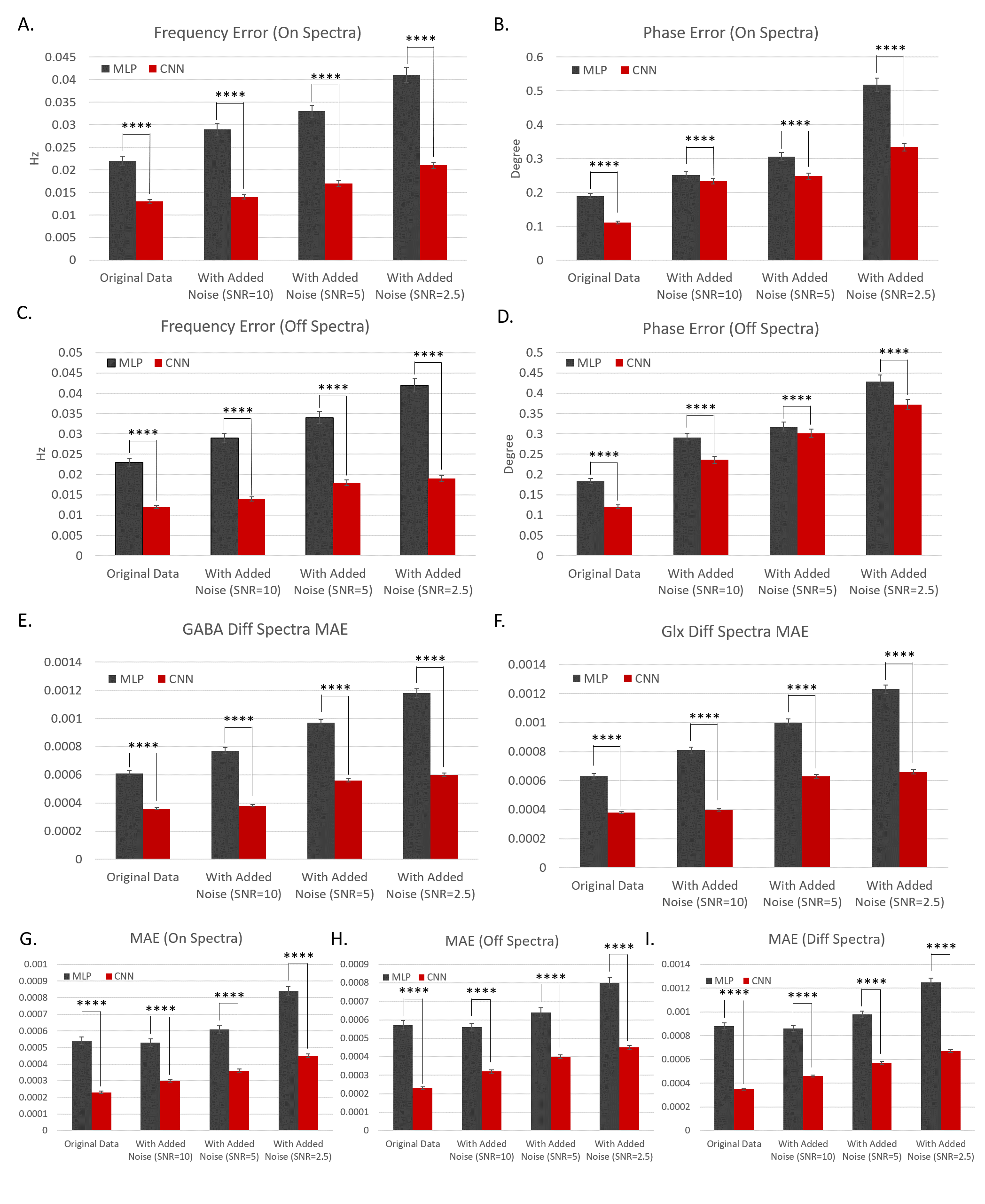
3.1. Spectra analysis and error comparison using the simulated dataset at varying SNRsThe CNN-based approach had smaller frequency and phase offset prediction errors. The mean frequency offset error and phase offset error was smaller using the CNN-based approach (0.01 ± 0.01 Hz and 0.12 ± 0.09°) compared to the MLP-based approach (0.02 ± 0.02 Hz and 0.19 ± 0.17°). At lower SNRs, the CNN-based approach performed better than the MLP-based approach as well (Ex. SNR=2.5: 0.01 ± 0.02 Hz and -0.07 ± 0.44° for CNN; 0.00 ± 0.05 Hz and 0.02 ± 0.61° for MLP). The results can be observed from Figure 2. Moreover, the CNN model had lower frequency and phase estimation errors than the MLP model for both the On and Off spectra at varying SNRs. Additionally, residual spectra errors in the GABA Diff spectra region, Glx Diff spectra region, Off spectra, On spectra and Diff spectra were found to be lower using our model. These results can be observed in Figure 3.
3.2. In vivo Dataset
From figure 4, with small offsets C1, all three methods (MLP, CNN and SR) performed similarly. As for medium offsets C2, the performance of the CNN-based approach and the MLP-based approach was comparable, but both models performed better than SR. When large offsets C3 were added, the performance of our model was better than the MLP-based approach and SR’s.
Discussion and Conclusion
From Figure 2 and 3, we observed that the CNN model performed better compared to the MLP model when using simulated data as smaller correction errors and residual errors were observed indicating CNNs are a better protocol for FPC. The standard deviation was smaller too. The influence of noise was also found to be smaller indicating CNNs are more robust. From Figure 4, better performance in the CNN model was observed where the output spectra were clearer and more robust to additional offsets when compared to the MLP-based approach. This result was also observed by its larger P and Q value with different additional offsets (no offset, C1, and C3).Using CNNs were found to demonstrate accurate quantification with training and validation for frequency and phase offset estimation in separate models. These observations show the utility the model has for MRS quantification. However, the CNN method takes more computational time to train the models and makes the method inflexible to account for additional parameters such as first-order phase, amplitude, and bandwidth variance in different transients. For future work, combining frequency and phase offset predictions into a single model can further improve computational efficiency.
Acknowledgements
This study was performed at the Zuckerman Mind Brain Behavior Institute at Columbia University and Columbia MR Research Center site.References
1. Gurbani SS, Schreibmann E, Maudsley AA, et al. A convolutional neural network to filter artifacts in spectroscopic MRI. Magn Reson Med. 2018;80(5):1765-1775. doi:10.1002/mrm.27166
2. Chandler, M.; Jenkins, C.; Shermer, S.M.; Langbein, F.C. MRSNet: Metabolite quantification from edited magnetic resonance spectra with convolutional neural networks. arXiv 2019, arXiv:1909.03836.
3. Tapper S, Mikkelsen M, Dewey BE, Zöllner HJ, Hui SCN, Oeltzschner G, Edden RAE. Frequency and phase correction of J-difference edited MR spectra using deep learning. Magn Reson Med. 2021 Apr;85(4):1755-1765. doi: 10.1002/mrm.28525. Epub 2020 Nov 18. PMID: 33210342.
4. Mullins PG, McGonigle DJ, O’Gorman RL, et al. Current practice in the use of MEGA-PRESS spectroscopy for the detection of GABA. Neuroimage 2014;86:43–52.
5. Near J, Edden R, Evans CJ, Paquin R, Harris A, Jezzard P. Frequency and phase drift correction of magnetic resonance spectroscopy data by spectral registration in the time domain. Magn Reson Med. 2015;73:44-50.
6. D. Kingma and J. Ba. Adam: A method for stochastic optimization”. arXiv 2014, arXiv:1412.6980.
Figures