4489
Optimizing Prostate DWI Acquisitions for non-Gaussian models using an Activity MRI [aMRI] library1Advanced Imaging Research Center, Oregon Health & Science University, Portland, OR, United States, 2Portland VA Medical Center, Portland, OR, United States, 3Urology, Oregon Health & Science University, Portland, OR, United States, 4Diagnostic Radiology, Oregon Health & Science University, Portland, OR, United States
Synopsis
Characterizing the non-Gaussian signature of the prostate DWI b-space decay often employs the kurtosis-, stretched-, and bi-exponential models. However, the optimal acquisition strategy in terms of maximum b value sampled and the number of b-values needed remains a research topic. Using the best-matched curves from a DWI library created with Monte Carlo random walk simulations of contracted Voronoi-cell ensembles, this work shows that, for prostate DWI, a maximum b-value near 2000 s/mm2 is optimal and the number of b-values is not as crucial as long as it is larger than the number of model parameters.
Introduction
Characterizing the non-Gaussian signature of prostate DWI b-space decay is gaining interest. However, effort on in vivo DWI acquisition optimization is somewhat limited due to the lack of an analytical or quantitative reference. We use the best-matched curves from a DWI library created with Monte Carlo random walk simulations in contracted Voronoi-cell ensembles.1,2 The goal of this work is to investigate the optimal extent of diffusion-weighting (maximum b-value), and the number of b-values desired, for prostate DWI acquisitions. Here, the prostate DWI non-Gaussian signature is quantified with kurtosis-3, stretched-4, and/or bi-exponential models.Methods
After informed consent, seven subjects underwent 3T (Siemens) prostate multi‑parametric MRI (mpMRI) with an endorectal RF coil. The DWI protocol employed a b-value range from 0 to 5,000 s/mm2. Other details are: 128 x 128 in-plane matrix (40% phase oversampling), 24 cm FOV, 3.0 mm slice thickness and ~5.7 min acquisition time. Five mp-MRI visible lesions from five subjects were confirmed by clinical biopsies. Lesion and contralateral normal appearing (NA) prostate tissue region-of-interests (ROIs) were drawn on de-noised5,6 DWIs. These ROIs were further grouped by Gleason scores (only GS6 and GS7) or NA tissue. Pixel-wise matching of b-space DWI decay curves with aMRI library entries7 was performed and the results assigned to the appropriate lesion-status groups. The aMRI library curve located at the center of all matched-curves within a group is then selected as the representative curve for that tissue. This results in a reference curve for each of the GS6, GS7, and NA tissues.
To determine optimal acquisition strategy on how many b-values [b-num] to acquire and what is the optimal largest b-value [bmax] to sample, 10 different b value numbers from 3 to 12, and 23 bmax values from 600 to 5,000 s/mm2 [step size 200] were used. These form a 10 x 23 grids in b-num, bmax space. The three curves selected (GS6, GS7 and NA) are fitted with kurtosis-, stretched-, and bi‑exponential-models for each b-num, bmax parameter combination. Because none of the empirical models can perfectly match the reference library curves, serial root-mean-square error (RMSE) calculated up to a pre-defined upper bound of b-value [bset, 1600 to 3200 s/mm2, step size 200 s/mm2] with fine‑sampled b-value array [0 to bset, step-size 10] are used to quantify the goodness of the matchings. Using a bmax of 2000 s/mm2 as an example, the fittings will employ b-num from 3 to 12 (kurtosis and stretched models) and 4 to 12 (bi-exponential model) for an evenly spaced b array from 0 to 2000 s/mm2. Then, both reference and fitted curves are fine-sampled, at 10 s/mm2 increment, to bset, which can be different than 2000 s/mm2.
Results
Figure 1a shows a de-noised DWI image for b = 5,000 s/mm2. Since multiple acquisition is unavailable, SNR (~ 22 for the case shown) was estimated using signal mean from a tissue ROI over the standard deviation derived from an ROI from an image area away from any tissue. Panel b shows the noise distribution histogram from the 1a rectangular noise ROI after the de-noising step. The near Gaussian distribution indicates the SNR estimation method is reasonable. Panel c shows pixel DWI data with the curves selected as their respective best-matches. The hashed area at the bottom demarks the estimated noise level of these data.Figure 2 shows the three selected curves (black, reference) and their respective kurtosis- (blue), stretched- (purple), and bi-exponential-model (brown) fittings. The modeling used a bmax of 2000 s/mm2, but the fine-sampled calculation extends to 3000 s/mm2, (bset = 3000 s/mm2). As expected, the best-fitted curves from all three models start to show noticeable departure from the reference tissue curves at b values above ~ 2500 s/mm2 when the fitting employed bmax of only 2000 s/mm2.
Figures 3-5 shows the natural log RMSE contours for kurtosis-, stretched-, and bi-exponential-models, respectively, for bset = 2400 s/mm2. It is interesting to notice that the overall accuracy of each of the three models is primarily determined by bmax, which is shown to have an optimal range of ~ 1800 – 2500 s/mm2 for the modeling. On the contrary, b-num is not as sensitive. Given the relatively small differences (compared to those introduced by DWI data with SNR ~ 20) shown in the RMSE contours, it is likely the overall trend seen in these plots will hold for noisy in vivo data. That is, the optimal bmax is in the low 2000 s/mm2, and b-num value is not as critical. It is also worth noting that this general pattern is observed when bset is varied from 1600 to 3200 s/mm2 (not shown), supporting the general conclusion that the bmax is a more important parameter of the two.
Discussion
Using best-matched diffusion library curves located at the center of each prostate tissue type ROI as references, this simulation shows that when the non-Gaussian signature of prostate DWI b‑space decay is quantified with kurtosis-, stretched-, and/or bi-exponential-models, the optimal maximum b-value is around 2000 s/mm2 and the number of b-values in the DWI acquisition is generally not as important. A limitation of the study is that it doesn’t contain lesion data for GS8 and above.Acknowledgements
Grant Support: Brenden-Colson Center for Pancreatic Care.
Oregon Clinical and Translational Research Institute, NIH/NCATS.
Thorsten Feiweier (Siemens) for providing the work-in-progress sequence for DWI data acquisition.
References
1. Baker, Moloney, Li, Gilbert, Springer, PISMRM, 27:3612 (2019).
2. Baker, Moloney, Li, Wilson, Barbara, Maki, Gilbert, Springer, PISMRM, 27:3585 (2019).
3. Jensen, Helpern, Ramani, Lu, Kaczynski, Magn. Reson. Med. 53:1432-1440 (2013).
4. Liu, Zhou, Peng, Wang, Zhang, J. Magn. Reson. Imaging. 42: 1078-1085 (2015).
5. Veraart J, Novikov DS, Christiaens D, Ades-Aron B, Sijbers J, Fieremans E. Neuroimage. 142:394-406 (2016).
6. Does, Olesen, Harkins, Serradas-Duarte, Gochberg, Jespersen, Shemesh. Magn Reson Med. 81:3503-3514 (2019).
7. Li, Baker, Moloney, Kopp, Coakley, Garzotto, Springer, PISMRM, 29:4097 (2021).
Figures
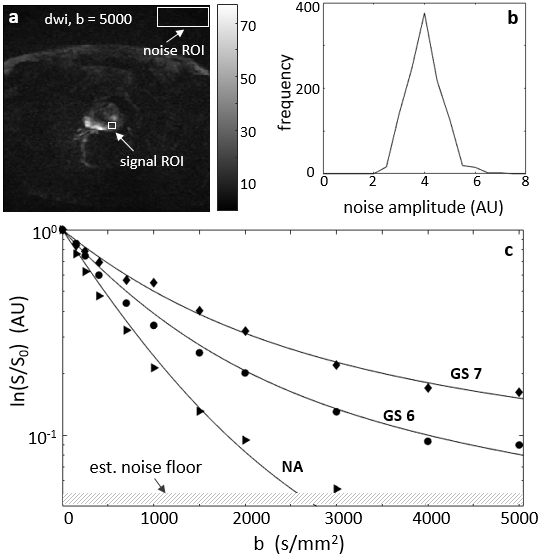
Figure 1. Panel a shows a de-noised DW image for b = 5,000 s/mm2. The signal and noise ROIs used for SNR estimation are shown as white rectangles. Panel b shows the noise distribution histogram after the de-noising step from the 1a rectangular noise ROI. The near Gaussian distribution indicates the SNR (~ 22) estimation approach is reasonable. Panel c shows pixel DWI data with the selected reference curves as their respective best matches. The hashed area at the bottom demarks the estimated noise level of these data.
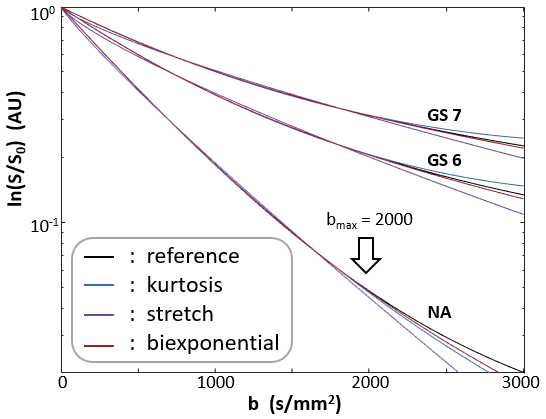
Figure 2. The three selected curves (reference, black) and their respective kurtosis- (blue), stretched- (purple), and bi-exponential-model (brown) best fittings. The modeling used a bmax value of 2000 s/mm2. The fine-sampled calculation, however, extends to 3000 s/mm2 (bset =3000 s/mm2). As expected, the best-fitted curves from all three models start to show noticeable departure from the reference tissue curves at b values above ~ 2500 s/mm2 - when bmax of only 2000 s/mm2 is used in the fittings.
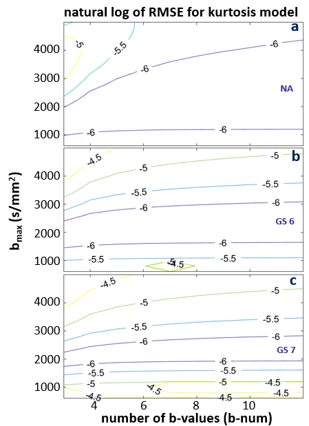
Figure 3. The natural log RMSE contours for the kurtosis model are shown for NA (a), GS6 (b), and GS7 (c) data, respectively. The more negative the natural log RMSE value, the smaller the error. RMSE values were calculated based on fine sampled data at a step-size of 10 s/mm2, with a range of 0 – 2400 s/mm2. The optimal bmax range is between ~1800 -2500, and the b-num (number of b-values) is not as sensitive. Similar patterns are seen for a wide range of bset from 1600 to 3200 s/mm2 (not shown).
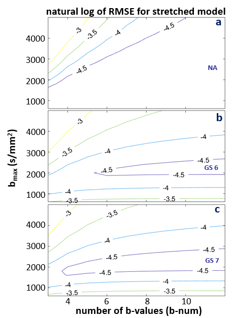
Figure 4. The natural log RMSE contours for the stretched model is shown for NA (a), GS6 (b), and GS7 (c) data, respectively. RMSE were calculated based on fine sampled data at a step-size of 10 s/mm2 and a b-range of 0 – 2400 s/mm2. The optimal bmax range is between ~1800 -2500. Even though a b-num of higher than 5 could be favored, the general trend of b-num is not as crucial as bmax is expected to remain true for noisy in vivo data. Similar patterns are seen for a wide range of bset from 1600 to 3200 s/mm2 (not shown).
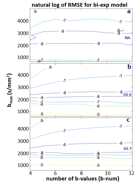
Figure 5. The natural log RMSE contours for the bi-exponential model is shown for NA (a), GS6 (b), and GS7 (c) data, respectively. RMSE were calculated based on fine sampled data at a step-size of 10 s/mm2, with a range of 0 – 2400 s/mm2. The optimal bmax range is between ~2000 -2500, and the b-num (number of b-values) is not as sensitive. However, since the bi-exponential model has one additional parameter, the lowest b-num starts at 4. These also give the smallest errors (best fit). Similar patterns are seen for a wide range of bset from 1600 to 3200 (not shown).