4447
Simultaneous estimation of longitudinal relaxation time and intracellular water lifetime using Active Contrast Encoding MRI1Weill Cornell Medical College, New York, NY, United States
Synopsis
Dynamic contrast enhanced (DCE)-MRI can be used as a tool to measure intracellular water lifetime (τi) in tumor cells which can be used as a biomarker for tumor aggressiveness and treatment response. Contrast kinetic model analysis in DCE-MRI requires accurate pre-contrast T1 measurement. We used multiple flip angles for active contrast encoding of both T1 and τi during dynamic data acquisition with one injection. The present study demonstrates the feasibility of measuring T1 and τi simultaneously from the active contrast encoding (ACE) MRI data. ACE-MRI also reduces the scan time by eliminating the need of separate pre-contrast T1 measurement.
Introduction
Tumor intracellular water lifetime (τi) has potential as a biomarker for tumor aggressiveness and treatment response. Previously, we demonstrated that using two flip angles in series during T1-weighted dynamic contrast enhanced (DCE)-MRI improves precision of τi measurement, compared to the conventional DCE-MRI data with single flip angle for the entire dynamic scan.1 However, it was necessary to measure pre-contrast longitudinal relaxation time (T10) separately before contrast injection. It was also found that τi is very sensitive to small variations in T10 value, including mismatch between T10 map and DCE-MRI data.1 Hence, in this study, we propose to use multiple flip angles in one DCE-MRI acquisition, i.e., active contrast encoding (ACE) MRI, for simultaneous estimation of T1 and τi. The proposed concept of ACE-MRI was tested using murine tumor models.Methods
Six to eight -week-old Fischer rats (n=3) with 9L gliosarcoma model were included in this study. MRI experiments were performed on Bruker 7T micro-MRI system, with four-channel phased array rat head receive-only MRI surface coil. DCE-MRI scan was performed using 3D-UTE-GRASP pulse sequence2 (TR=5ms and TE=0.028ms) to achieve an isotropic spatial resolution and to minimize the T2* effect. It was continuously run to acquire 135,800 spokes (9,700 spokes each flip angle segment, total 14 segments, flip angels of segments in series were: 10o - 10 o - 10 o - 10 o - 2 o - 10 o - 20 o - 10 o - 5 o - 10 o - 15 o - 10 o - 25 o - 10 o) for 11 min 19 s. Image reconstruction was conducted to have temporal frame resolution T= 2.5 s/frame, Image matrix = 128x128x128, field of view = 37x37x37 mm and the spatial resolution was 0.289x0.289x0.289 mm. A bolus of gadobutrol (Gadavist, Bayer) in saline at the dose of 0.1 mmol/kg was injected through a tail vein catheter, starting 60 seconds after the start of data acquisition. Prior to the DCE-MRI experiment, a 3D T1 map with the same isotropic high resolution was obtained using the same 3D-UTE-GRASP sequence3 with variable flip angles (2o - 4 o - 6 o - 8 o - 10 o - 12 o, 6,960 spokes for each flip angle, with total acquisition time was 209 s), for comparison with the proposed method that does not use the pre-contrast T1 mapping data. Arterial Input Function (AIF) was obtained using the median of the 10 most enhancing vessels (selected by initial area under curve, IAUC) from the whole head. For AIF signal intensity to concentration conversion, the T1 values of those vessels were obtained by minimizing the jumps in the concentration curve as demonstrated before.1 First, pharmacokinetic model analysis was carried out with the two-compartment exchange model with water exchange1,4 using pre-contrast separately measured T10, estimating five parameters: PS (permeability surface area product), Fp (blood flow), ve (extracellular space volume fraction), vp (vascular space volume fraction) and τi (intracellular water lifetime); this approach was denoted as 5P. Then, by incorporating T10 as an additional free parameter in the model instead of using measured T10, pharmacokinetic model analysis was repeated for six parameter estimations, T10, PS, Fp, ve, vp, and τi; hence this approach was denoted as 6P, i.e., six parameters fitting for simultaneous T10 and τi measurement.Results and Discussions
Figure 1A and 1B show 3D rendering of the pre-contrast T1 map with the same isotropic resolution as DCE-MRI scan and T1 maps of one slice in axial/coronal/sagittal planes. Figure 1C showed the maximum intensity projections of the DCE-MRI frames acquired. Figure 2A and 2B show the signal enhancement curves of the selected 10 most enhancing voxels and the converted concentration curve as the AIF used for pharmacokinetic model analysis. Figure 2C and 2D showed example curve fits for one tumor voxel using 5P and 6P methods, respectively. The fitting performance were reasonable despite the signal intensity jumps along the washout portion with multiple flip angles. This was observed with most voxels. Figure 3 shows comparisons of parameter maps between the 5P and 6P methods for tumor center slices in axial/sagittal/coronal planes. It clearly shows that all the parameters are in good agreement between two approaches in terms of absolute value range and spatial patterns. Figure 4 shows the boxplots of the parameters for comparison between the 5P and 6P methods. The median and inter-quartile-range (IQR) of all the parameters were (5P median/IQR, 6P median/IQR): T1 (1.899/0.179 s and 1.895/0.204 s), ve (0.157/0.053 and 0.156/0.055), vp (0.030/0.020 and 0.031/0.022), PS (0.043/0.044 /min and 0.042/0.044 /min), Fp (1.321/2.057 /min and 1.255/2.096 /min), and τi (1.181/1.105 s and 1.178/0.996 s). Figure 5 summarized the comparison from all the animals.Conclusion
This study demonstrates the feasibility of using ACE-MRI with six flip angles for simultaneous estimation of T1 and τi. While the pharmacokinetic parameters were found consistent through the entire tumor volumes between 5P (without T10 estimation) and 6P (with T10 estimation), our results show that the τi had a relatively weaker correlation, which was likely caused by small degree of disagreement in T1 measurement. Future study will focus on optimizing the scan protocol in terms of the number of flip angles, duration of flip angle segment and total scan time toward applying this approach for assessment of tumor aggressiveness and treatment response.Acknowledgements
NIH R01CA160620, R01CA219964, UH3CA228699.References
- Zhang J, Kim S. Estimation of cellular-interstitial water exchange in dynamic contrast enhanced MRI using two flip angles. NMR in Biomedicine, 2019 Nov;32(11),e4135
- Zhang J, Feng L, et al. Rapid dynamic contrast-enhanced MRI for small animals at 7T using 3D ultra-short echo time and golden-angle radial sparse parallel MRI. MRM, 2019 Jan;81(1):140-152.
- Zhang J, Kiser K, et al. Fast 3D T1 mapping with isotropic high resolution using ultrashort TE MRI. ISMRM 2020 abstract #4709
- Sourbron SP, Buckley DL. Tracer kinetic modelling in MRI: estimating perfusion and capillary permeability. Phys Med Biol. 2012 Jan 21;57(2):R1-33
Figures
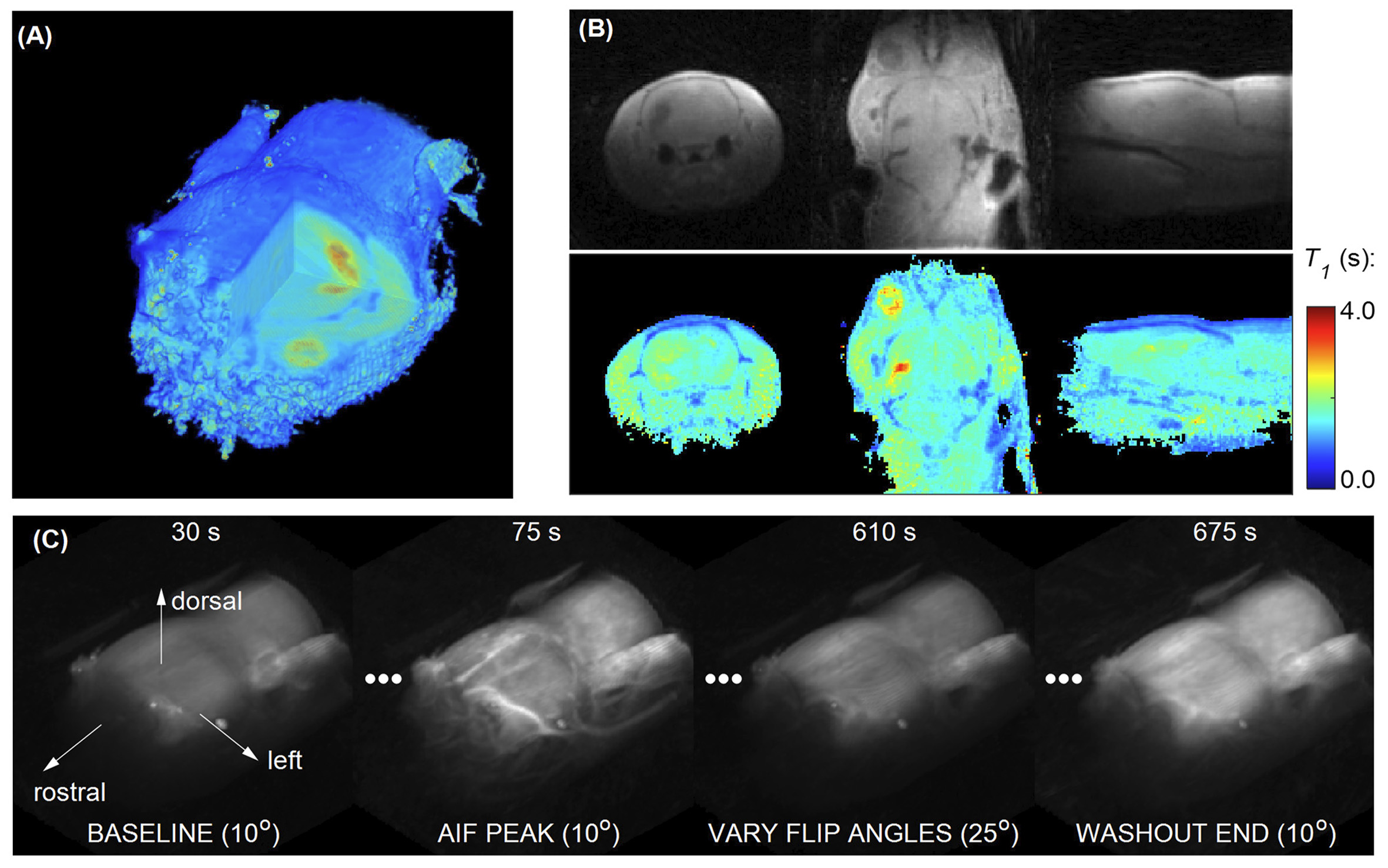
Figure 1. Pre-contrast T1 maps and DCE-MRI frame. (A) 3D T1 map with isotropic resolution measured with 3D-UTE-GRASP and variable flip angle method. (B) T1 maps in axial/coronal/sagittal planes. (C) DCE-MRI frames at baseline, AIF peak and washout end (acquired with baseline flip angle of 10o), and one frame with flip angle of 25o. Frames acquired with other flip angles are not shown here.
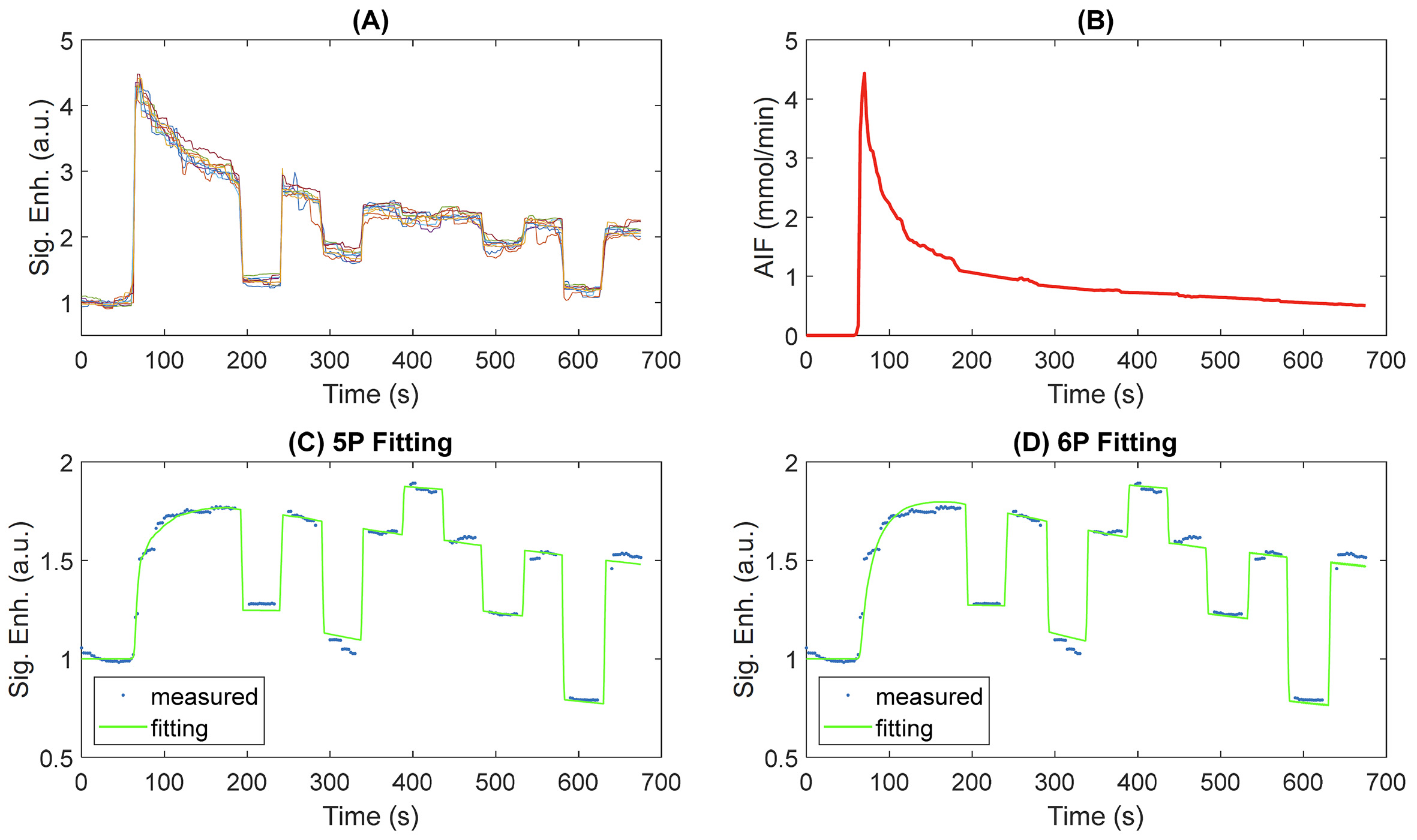
Figure 2. AIF and sample fittings. (A) Signal intensity curves of the most enhancing 10 vessels. Signal jumps in washout region correspond to the different flip angles used. (B) AIF obtained using median of the 10 vessels by converting signal intensity to concentration. Though there were jumps in signal intensity, AIF concentration remained continues. Demonstration fittings of one tumor voxel with 5P (ve/vp/PS/Fp/τi) fitting (C) and 6P (included one more parameter, T10) fitting (D).
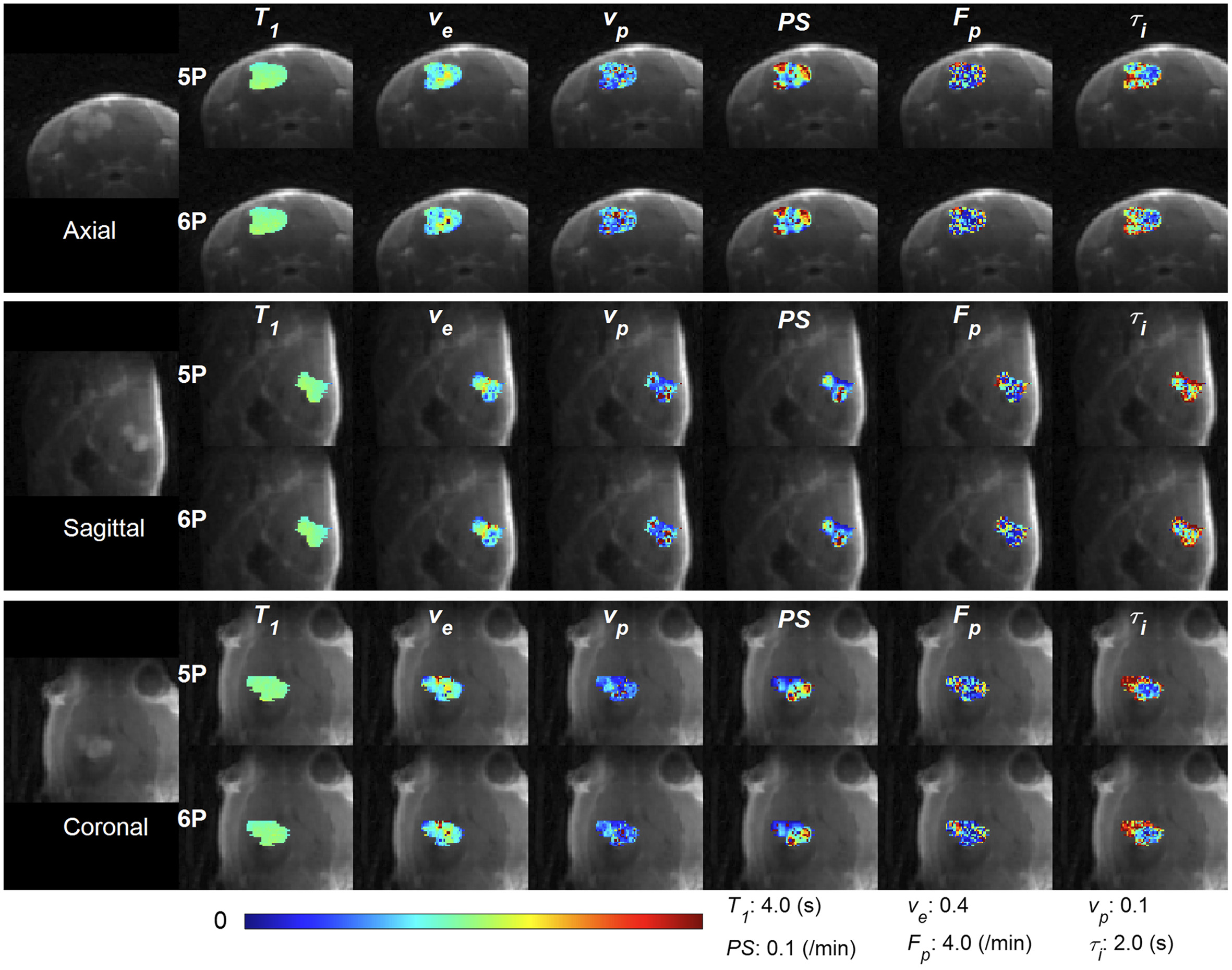
Figure 3. Parameter color maps of 5P (with measured T10) and 6P fitting in axial/sagittal/coronal planes with background images in each direction.
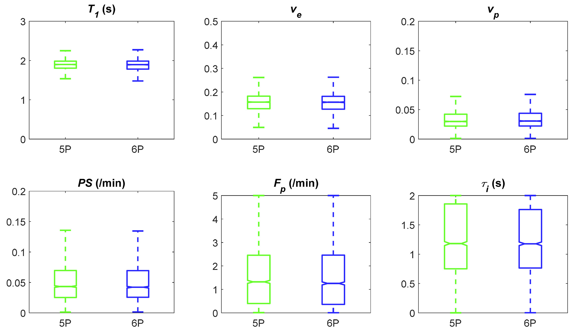
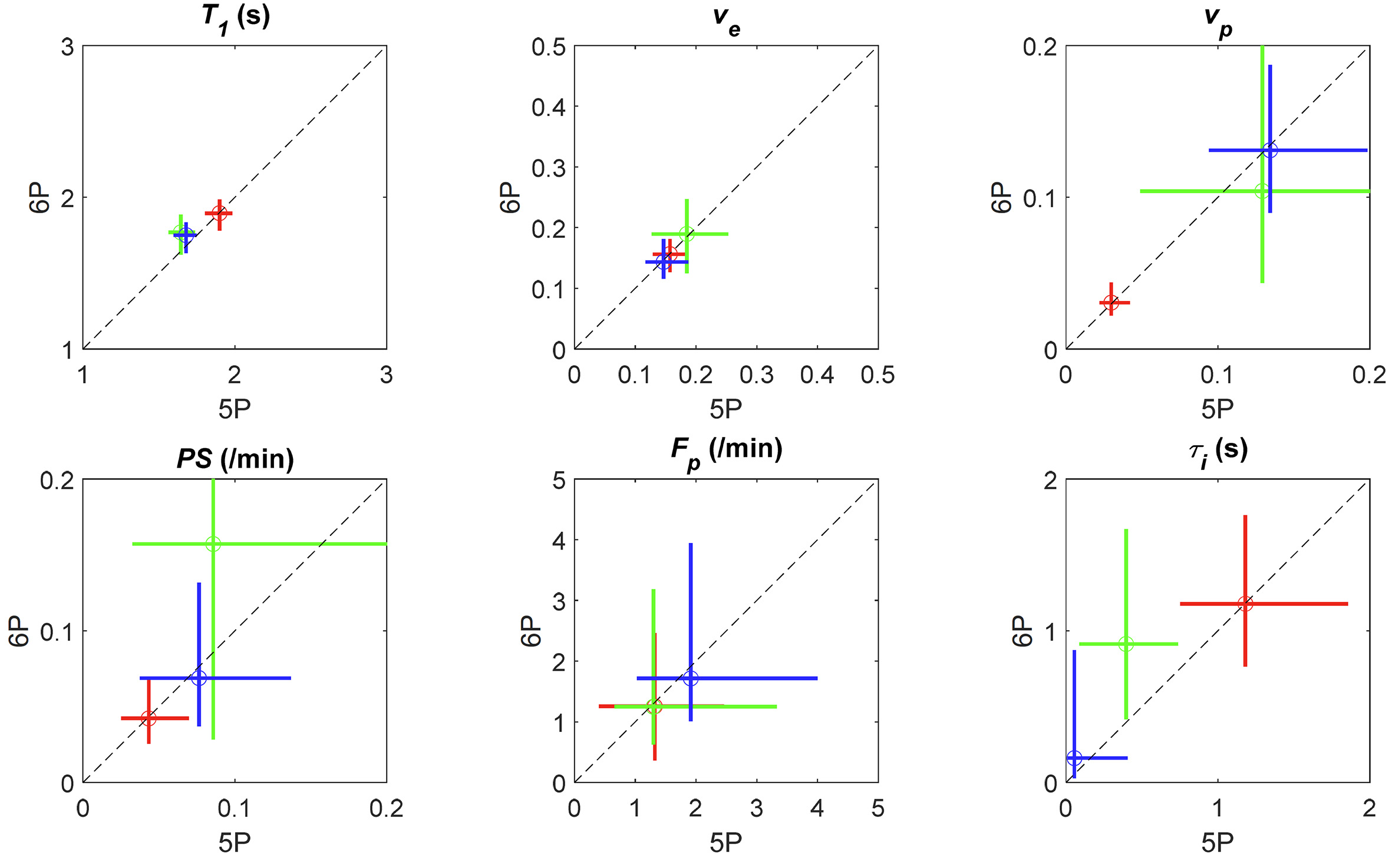
Figure 5. Comparison of tumor parameters between 5P (with measured T10) and 6P fitting using multiple animals. Each color represents one animal. The circles represent the median values, and the length of the colored lines represents the 25%~75% range of each method.