4440
Free-running Simultaneous 3D Cardiac T1 Mapping and Cine Imaging Using a Linear Tangent Space Alignment Model1Gordon Center for Medical Imaging, Department of Radiology, Massachusetts General Hospital, Harvard Medical School, Boston, MA, United States, 2LTCI, Telecom Paris, Institut Polytechnique de Paris, Paris, France, 3LIP6, Sorbonne University, CNRS, Paris, France
Synopsis
Cardiac T1 mapping allows assessment of tissue characteristics and functioning of the heart. However, existing methods are limited in terms of spatial resolution and coverage due to limitations in acquisition speed and the presence of cardiac and respiratory motion. This work proposes a new reconstruction framework for simultaneous, high-resolution 3D cardiac T1 mapping and cine imaging of the heart at 3T from sparsely sampled k-space data.
Introduction
Cardiac T1 mapping is a powerful magnetic resonance (MR) imaging technique that allows quantitative assessment of tissue characteristics and underlying pathology of the myocardium1. Up to date, various methods have been developed to overcome the limitations due to cardiac and respiratory motion and enable cardiac T1 mapping with free-breathing acquisitions2-5. However, existing methods are still limited in terms of imaging speed, spatial resolution and coverage (i.e., in the slice selection direction). In this work, we propose a new method to enable free-running (i.e., free-breathing and no ECG gating), simultaneous 3D cardiac T1 mapping and cine imaging using a linear tangent space alignment (LTSA) model. The performance of the proposed method is validated using in vivo experimental data obtained from healthy volunteers at 3T.Method
Image ReconstructionThe data is reconstructed using the Linear Tangent Space Alignment (LTSA) model6. Consider the Casorati matrix of the dynamic image series $$$X=[x_1,...,x_N]\in{\mathbb{C}^{M\times{N}}}$$$ (M is the number of voxels and N the number of frames) sampled from a low-dimensional manifold $$$\mathcal{M}$$$. The images $$${x_i}$$$ can be grouped into $$$C$$$ neighborhoods based on a similarity metric, forming $$$X_c=[x_{i^{(c)}_{1}},...,x_{i^{(c)}_{K_c}}]\in{\mathbb{C}^{M\times{K_c}}}$$$ where $$${i^{(c)}_{k}}$$$ corresponds to the frame index of the $$$k$$$-th image at the $$$c$$$-th neighborhood and $$$K_c$$$ to the total number of frames in that neighborhood. The LTSA model for the neighborhood $$$c$$$ is then:
$$X_c=T{L}_c^{-1}{\Phi}_c^T$$
Where $$$T\in{\mathbb{C}^{M\times{d}}}$$$ is composed of the global coordinates of the underlying manifold $$$\mathcal{M}$$$, $$${L}_c^{-1}\in{\mathbb{C}^{d\times{d}}}$$$ is a linear transformation matrix for the neighborhood $$$c$$$ and $$${\Phi}_c\in{\mathbb{C}^{{K_c}\times{d}}}$$$ is a matrix forming an orthonormal basis of the subspace of the neighborhood $$$c$$$. Note that $$${\Phi}_c$$$ can be learned from training data. The LTSA model is a nonlinear generalization of the conventional subspace models (i.e., the low-rank and low-rank tensor models). It leverages the intrinsic low-dimensional structure of the dynamic MRI images for accelerated real-time imaging with sparse sampling.
In image reconstruction, we minimize the representation error of $$$T$$$ and $$$\left\{L_c^{-1}\right\}_{c=1}^C$$$ with a sparsity constraint on $$$T$$$:
$$arg\min_{T,\left\{{{L}_c}^{-1}\right\}_{c=1}^C}\Big\{\frac{1}{2}\sum_{c=1}^C{||A_c\{T{L}_c^{-1}{\Phi}_c^T\}-s_c||_2^2}+{\lambda}_1||DT||_1\Big\}$$
where, $$$s_c$$$ is the undersampled k-space data of the neighborhood c, $$$A_c$$$ is the forward imaging matrix, $$$D$$$ is the finite difference operator along (x,y,z) directions and $$$\lambda_1$$$ is a scaling parameter for the sparsity constraint. This optimization problem is solved using the alternating direction methods of multipliers (ADMM) algorithm7.
We seek to form neighborhoods such that the matrices $$$X_c,c=1,\ldots,{C}$$$ have each a low modelling rank. As shown in [4], forming neighborhoods based on respiratory motion is a good candidate for that purpose. Therefore in this work, we form $$$X_c$$$ with images belonging to the same respiratory phase.
In Vivo Study
Experiments were performed on a 3T MR scanner. In vivo experiments were performed on a healthy volunteer (approved by our local IRB) using a free-running continuous acquisition sequence with spoiled gradient-recalled echo (GRE) readout and adiabatic inversion pulse (Fig. 1b). A special data acquisition scheme was employed to sample data along a stack-of-stars trajectory (Figs. 1b and c) and enable image reconstruction using the LTSA model8. One study was performed using the following imaging parameters: FOV=300×300×128 mm3, matrix-size=160×160×32, TR/TE=5.5/2.0 ms, flip-angle=5°, number-of-TRs-per-frame=9, time-between-IR-pulses=1528 ms, and acquisition time=~12.4 min. Another study was performed to achieve higher spatial resolution and coverage with all other imaging parameters the same: FOV=300×300×160 mm3 and matrix-size=160×160×64. For comparison, 2D T1 maps were acquired using MOLLI9 in three slices in the short-axis view from the apical, mid-cavity, basal regions of the heart and for one slice in the long-axis view.
Estimation of $$$T_1$$$ was performed by first estimating the $$$T_1^{*}$$$ for each voxel via least-squares fitting of the inversion recovery signal to the following signal equation:
$$S[n]=A\cdot{}exp\Big(-\frac{n\cdot{}T_{frame}}{T_1^{*}}\Big)+B,\quad{n=0,\ldots,N-1}$$
where $$$S$$$ denotes the signal, $$$n$$$ denotes the inversion-time index, $$$T_{frame}$$$ denotes the temporal resolution of each frame, and $$$A$$$ and $$$B$$$ denote linear coefficients. Once $$$T_1^{*}$$$ was estimated, $$$T_1$$$ was estimated using the following equation:
$$T_1=\frac{1}{\frac{1}{T_1^{*}}+\frac{log(cos(\alpha\cdot{}B_1))}{TR}}$$
where $$$\alpha$$$ denotes the flip angle and $$$B_1$$$ denotes the transmit B1. In this work, uniform transmit B1 was assumed which was determined by calibrating the $$$T_1$$$ of the myocardium to literature value.
Results
Images reconstructed using LTSA showed fewer artifacts compared to those from low-rank plus sparsity-based image reconstruction as shown in Fig. 2. Figure 3 shows the LTSA-reconstructed images along different axes, demonstrating the capability of the proposed method in spatial coverage and in revealing respiratory motion, cardiac motion (with synthesized bright- and dark-blood contrasts) and contrast changes during inversion recovery. The 3D T1 maps (12 out of 32 slices) from the proposed method were comparable to those acquired from MOLLI (Fig. 4). The myocardium T1 was 1208.7 ± 60.0 ms for MOLLI and 1189.8 ± 168.9 ms for proposed method. Figure 5 shows our preliminary results when pushing the proposed method to achieve a spatial resolution of 1.9x1.9x2.5 mm3 (64 slices) in a 12-min acquisition.Conclusion
A new method is proposed to achieve simultaneous 3D T1 mapping and cine imaging of the heart using a linear tangent space alignment-based image reconstruction.Acknowledgements
This work was supported in part by the National Institutes of Health (P41EB022544, R01CA165221, R01HL137230, and K01EB030045).References
1. Messroghli DR et al. "Clinical recommendations for cardiovascular magnetic resonance mapping of T1, T2, T2* and extracellular volume: a consensus statement by the Society for Cardiovascular Magnetic Resonance (SCMR) endorsed by the European Association for Cardiovascular Imaging (EACVI)." Journal of Cardiovascular Magnetic Resonance. 2017; 19(1):1-24.
2. Qi, Haikun, et al. "Free‐running 3D whole heart myocardial T1 mapping with isotropic spatial resolution." Magnetic resonance in medicine 82.4 (2019): 1331-1342.
3. Christodoulou, Anthony G., et al. "Magnetic resonance multitasking for motion-resolved quantitative cardiovascular imaging." Nature biomedical engineering 2.4 (2018): 215-226.
4. Hamilton, Jesse I., et al. "Cardiac cine magnetic resonance fingerprinting for combined ejection fraction, T1 and T2 quantification." NMR in Biomedicine 33.8 (2020): e4323.
5. Milotta, Giorgia, et al. "3D whole‐heart isotropic‐resolution motion‐compensated joint T1/T2 mapping and water/fat imaging." Magnetic Resonance in Medicine 84.6 (2020): 3009-3026.
6. Y. Djebra, I. Bloch, G. El Fakhri, C. Ma, “Manifold learning via tangent space alignment for accelerated dynamic MR imaging with highly undersampled (k,t)-data”, International Society for Magnetic Resonance in Medicine, June 2021.
7. S. Boyd et al, “Distributed optimization and statistical learning via the alternating direction method of multipliers,” Foundations and Trends in Machine Learning, vol. 3, no. 1. pp. 1–122, 2010.
8. Liang, Zhi-Pei. "Spatiotemporal imaging with partially separable functions." 2007 4th IEEE international symposium on biomedical imaging: from nano to macro. IEEE, 2007.
9. Kellman P et al. “Extracellular volume fraction mapping in the myocardium, part 1: evaluation of an automated method”. Journal of Cardiovascular Magnetic Resonance 2012; 14(1):1-11.
Figures
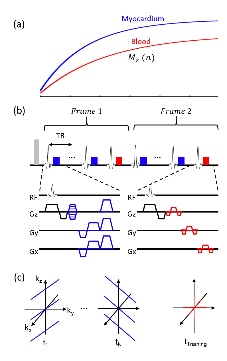
Figure 1. Schematic diagram of data acquisition. A: Illustration of inversion recovery of magnetization signal from myocardium and blood. B: Sequence for data acquisition. Data was acquired using a free-running (i.e., no cardiac or respiratory gating) continuous acquisition sequence with spoiled gradient-recalled echo (GRE) readout and inversion recovery. Imaging (blue) and training (red) datasets were acquired for image reconstruction. C: Example data acquisition for acquiring imaging and training datasets following radial stack-of-stars trajectory.
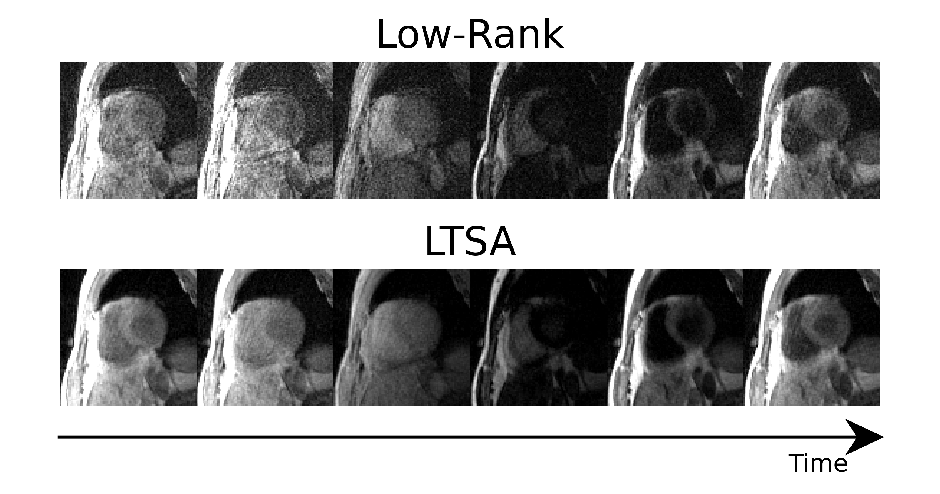
Figure 2. Comparison of reconstructed images between low-rank and LTSA reconstructions (both with sparsity constraint) . Reconstructed images over clock-time are shown. Notice the improvement in image quality using LTSA over low-rank reconstruction.
Figure 3. Animation of reconstructed images. Reconstructed images showing slice coverage (first column), respiratory motion (second column), cardiac motion with bright-blood contrast (third column), cardiac motion with dark-blood contrast (fourth column), and different contrast (fifth column).
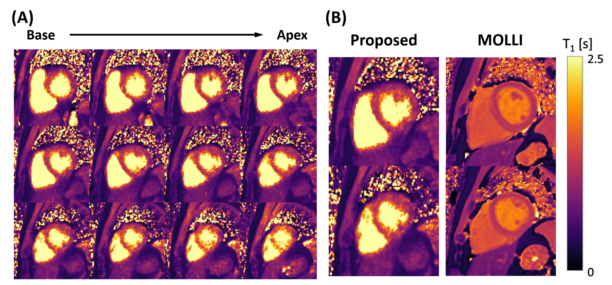
Figure 4. T1 mapping result from the 1st study. A: 3D T1 map estimated using the proposed method. B: T1 map comparison with 2D MOLLI acquisition.
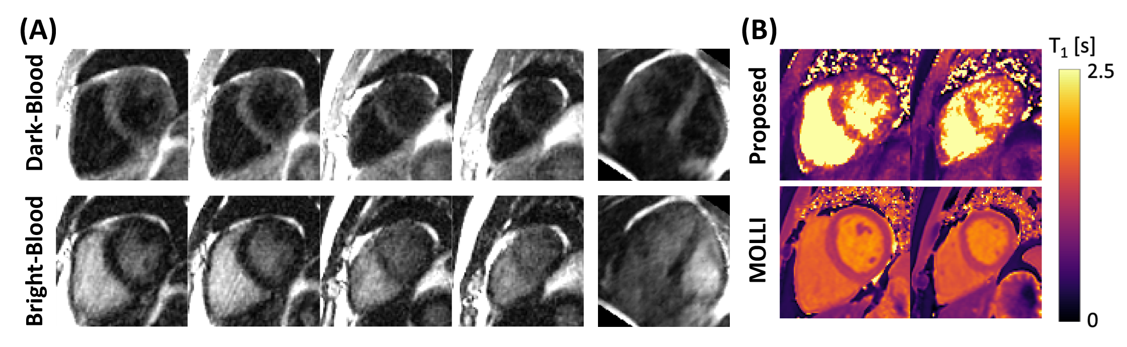
Figure 5. Result from 2nd study aiming for higher spatial resolution and coverage. A: Synthesized 3D images of the heart for dark- and bright-blood contrast. B: Estimated 3D T1 maps from the proposed method.