4413
In silico uncertainty quantification of the wall shear stress computed from phase-contrast 4d flow measurements.1Institute for Mathematical and Computational Engineering, Pontificia Universidad Católica de Chile, Santiago, Chile, 2Millennium Nucleus Center for the Discovery of Structure in Complex Data, Santiago, Chile, 3Department of Applied and Computational Mathematics and Statistics, University of Notre Dame, Notre Dame, IN, United States, 4Institute for Biological and Medical Engineering, Pontificia Universidad Católica de Chile, Santiago, Chile, 5Millennium Nucleus for Cardiovascular Magnetic Resonance, Santiago, Chile, 6Biomedical Imaging Center, Pontificia Universidad Católica de Chile, Santiago, Chile
Synopsis
The wall shear stress (WSS) is a relevant biomarker associated with the rupture of atherosclerotic plaques that can be computed from blood flow velocity measurements. We study the effect of noise velocity on the quantification of the WSS with a focus on the spatial correlations that may arise. We perform in silico experiments in which we consider a Hagen-Poiseuille flow and two noise distributions. Our results show evidence on the existence of spatial correlations in the WSS even when the velocity noise is uncorrelated.
Introduction
In the cardiovascular system, the vessel walls are constantly exposed to stress due to blood flow1,2. The wall shear stress (WSS) is defined as the force per unit area exerted on the vessel wall by blood flow3, and has been found to be a relevant biomarker when detecting the formation and rupture of atherosclerotic plaques1,2. The WSS can be computed from the flow velocities3. Non-invasive techniques, such as phase-contrast (PC) 4D flow4,5,6,7, allow us to compute the flow velocity during the cardiac cycle, which then can be used to quantify parameters such as the WSS5,6. The acquisition process in 4D flow has several sources of noise, ranging from electronic noise8 or involuntary movements of the patient9 to errors due to interpolation in the reconstruction of the magnetic resonance signal10. Although the noise in flow velocities has been studied6,7, its effect on the WSS has not received much attention. Even if the noise in the flow velocities may be uncorrelated, the noise in the WSS may be correlated, producing spatially coherent patterns that may lead to an inaccurate estimation of the WSS. The purpose of this work is to show numerical evidence that such spatial correlations in the WSS exist.Model
Fluid motion is governed by the Navier-Stokes equations. For Newtonian fluids, the surface stress tensor depends on pressure, viscosity and the velocity gradients. In a laminar flow on a cylindrical tube, the velocity gradient is due to the frictional forces exerted between the adjacent layers of the fluid and the walls of the conduit3. Therefore, the WSS is computed as the tangential force per unit area applied by the flow on the tube wall. Due to conservation of momentum, the WSS can be computed as $$\sigma = -P+ \mu (\nabla\vec{v}+\nabla\vec{v}^T)$$ where $$$\sigma$$$ represents the stress tensor, $$$P$$$ the pressure, $$$\mu$$$ is the fluid’s viscosity, and $$$\vec{v}$$$ is the fluid’s velocity. Note the WSS is represented as a vector that is tangent to the vessel’s boundary.Experimental Setup
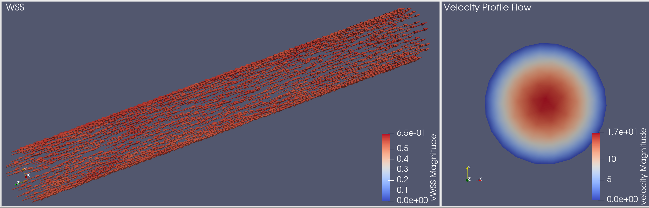
To study in silico the distribution of the WSS, we consider a Hagen-Poiseuille flow3 with maximum velocity 15.92 cm/s on a cylinder of radius 2 cm and length 24 cm. The WSS can be computed in closed-form3. Fig. 1 shows the true flow and WSS for a mesh with 1,500 nodes on the surface. We consider two distributions for the noise in the velocities. The first is additive Gaussian noise. In this case, the WSS has a multivariate normal distribution which is amenable to analysis. The second distribution, which we call PC-noise, arises in PC 4D flow. In this case, the flow is computed from the phases of 4 complex-valued images which are themselves corrupted by additive Gaussian noise6. Although the distribution of the WSS does not have a closed-form, numerical simulations will allow us to study the presence of spatial correlations in this case. Note in both cases the noise is Gaussian, the difference being whether it is applied to the velocities or to the complex-images.Results
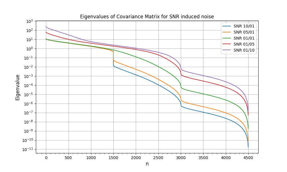
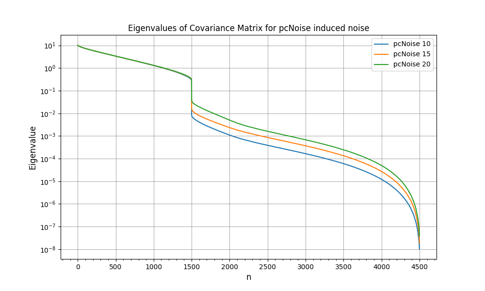
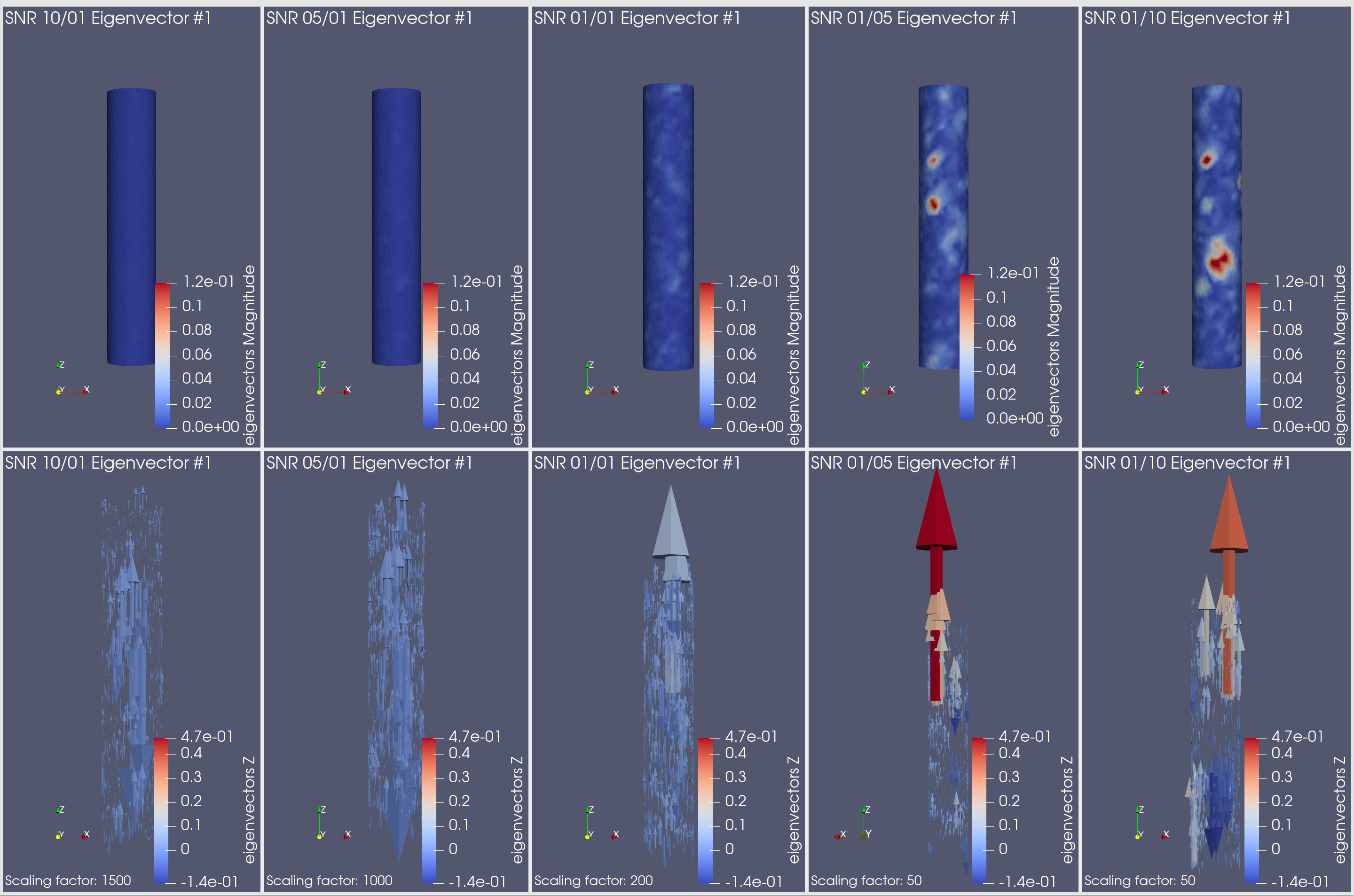
The noise was sampled from a Gaussian distribution with standard deviation $$\sigma_V = \frac{\sqrt{2} V_{\text{ENC}}}{\pi\text{SNR}}$$ characterized by the velocity-to-noise ratio, where $$$V_{\text{ENC}}$$$ is the velocity encoding and the SNR is the desired signal-to-noise ratio6,7. For the additive Gaussian noise distribution, we considered five values for the SNR, varying from 10 to 0.1. For PC-noise, we considered 3 values for the velocity encoding: 1, 1.5 and 2 times the maximum velocity. In each of the eight cases we simulated 4,600 samples to then subtract the true WSS and compute both the bias and the empirical covariance matrix. Then, we computed the eigendecomposition of the empirical covariance matrix, i.e., the Karhunen-Loève decomposition of the process11. Figs. 2 and 3 show the decay of the eigenvalues in each case. Their fast decay rate indicates the fluctuations of the WSS lie on a low-dimensional space, suggesting the presence of spatial correlations. Since the process can be simulated as a random combination of eigenvectors, mapping the leading eigenvectors to the cylinder surface shows the spatial correlations that appear in the WSS. Figs. 4 and 5 show the first eigenvector mapped to the cylinder surface for additive Gaussian noise and PC-noise. The magnitude of the WSS shows oscillatory spatial patterns, whereas the variations in the axial component indicate the WSS will be underestimated in some regions of the vessel wall and overestimated in others. Therefore, this suggests there may be spatial correlations in the WSS that may lead to an incorrect evaluation of the stress in the vessel wall.Conclusion
Our numerical results provide evidence of the existence of spatial correlation in the WSS, even when the noise in the flow velocity is uncorrelated. This behavior is observed both for additive Gaussian noise, or the noise arising from PC 4D flow acquisitions. This suggests these correlations should be studied further, to better understand the effect that noisy velocity measurements have on the accurate measurement of this biomarker. Future work will validate the presence of these fluctuations in anatomically realistic phantoms.Acknowledgements
This publication has received funding from ANID – Millennium Science Initiative Program – grant Nucleus for Cardiovascular Magnetic Resonance NCN17_129, from ANID – Millennium Science Initiative Program – Nucleus Center for Discovery of Structure in Complex Data NCN17_059, ANID – FONDECYT – 1211643, a Luksic Family Collaboration Grant, years 2018 and 2021, from Notre Dame International, a Luksic Family Collaboration Grant, year 2021, from Pontificia Universidad Católica de Chile, and an Open Seed Fund 2020 between the School of Engineering, Pontificia Universidad Católica de Chile and the Department of Applied and Computational Mathematics, University of Notre Dame.References
1. Mongrain, R. & Rodés-Cabau, J. (2006). Role of Shear Stress in Atherosclerosis and Restenosis After Coronary Stent Implantation. Revista Española de Cardiología. 59(1):1-4.
2. Samady, H., Eshtehardi, P., McDaniel, M. C., Suo, J., Dhawan, S. S., Maynard, C., Timmins, L. H., Quyyumi, A. A., Giddens, D. P. (2011). Coronary Artery Wall Shear Stress Is Associated With Progression and Transformation of Atherosclerotic Plaque and Arterial Remodeling in Patients With Coronary Artery Disease. Circulation. 124:779-788.
3. Katritsis, D., Kaiktsis, L., Chaniotis, A., Pantos, J., Efstathopoulos, E., Marmarelis, V. (2007). Wall Shear Stress: Theoretical Considerations and Methods of Measurement. Progress in Cardiovascular Diseases. 49(5): 307-309.
4. Sotelo, J., Dux-Santoy, L., Guala, A., Rodríguez-Palomares, J., Evangelista, A., Sing-Long, C., Urbina, J., Mura, J., Hurtado, D. E., Uribe, S. (2018). 3D axial and circumferential wall shear stress from 4D flow MRI data using a finite element method and a laplacian approach. Magnetic Resonance in Medicine. 79(5):2816-2823. doi: 10.1002/mrm.26927. Epub 2017 Oct 4. PMID: 28980342.
5. Hope, M. D., Hope, T. A., Crook, S. E., Ordovas, K. G., Urbania, T. H., Alley, M. T., & Higgins, C. B. (2011). 4D flow CMR in assessment of valve-related ascending aortic disease. JACC. Cardiovascular imaging, 4(7): 781–787.
6. Irarrazabal, P., Dehghan Firoozabadi, A., Uribe, S., Tejos, C., Sing-Long, C. (2019) Noise estimation for the velocity in MRI phase-contrast. Magnetic Resonance Imaging, 63:250-257. doi: 10.1016/j.mri.2019.08.028.
7. Nilsson A, Markenroth Bloch K, Carlsson M, Heiberg E, Ståhlberg F. Variable velocity encoding in a three-dimensional, three-directional phase contrast sequence: Evaluation in phantom and volunteers. J Magn Reson Imaging. 2012 Dec;36(6):1450-9. doi: 10.1002/jmri.23778. Epub 2012 Oct 12. PMID: 23065951.
8. Dwight G. Nishimura. Principles of Magnetic Resonance Imaging. Stanford University, 2010.
9. Krupa, K., & Bekiesińska-Figatowska, M. (2015). Artifacts in magnetic resonance imaging. Polish Journal of Radiology, 80, 93–106.
10. Hensley, L., Schiavazzi, D. E., Sing Long, C.A. (2021). Uncertainty and Undersampling with Applications to 4D Flow Magnetic Resonance Imaging. (manuscript in preparation).
11. Pavliotis, G. A. Stochastic Processes and Applications: Diffusion Processes, the Fokker-Planck and Langevin Equations. Springer, 2014.
Figures