Introduction

Tissue strain has gained increasing interest for assessing the function of several organs and has been extensively used due to its robustness and high reproducibility¹. However, tissue strain can be affected by the off-resonance effects of several chemical species but particularly the fat.

In this investigation, we study the effects of different fat fractions on strain estimated from tagged MR images using an in-silico phantom with a signal composed by two chemical species: water and fat.

Theory and methods

Signal model
We consider the case of two chemical species: water and fat. Let $$$\rho_W(\boldsymbol{X}) \leq 1$$$ and $$$\rho_F(\boldsymbol{X})=1-\rho_W(\boldsymbol{X})$$$ be the concentration of water and fat respectively. The signal of a tagged MR image at discrete time in presence of fat is given by:
$$
I^{tag}(\boldsymbol{X},t_k) = \rho_W(\boldsymbol{X}) I^{tag}_W(\boldsymbol{X},t_k) + \rho_F(\boldsymbol{X}) I^{tag}_F(\boldsymbol{X},t_k)
$$
where $$$I^{tag}_W$$$ and $$$I^{tag}_F$$$ represent the tagged signal of the water and fat respectively. In this investigation we considered the signal of Complementay Spatial Modulation of Magnetization (CSPAMM) images²:
$$
I^{tag}_W(\boldsymbol{X},t_k) = f_2(t_k,\alpha,T1_W,M_0)\{\cos(k_e X) + \cos(k_e Y)\} \\
I^{tag}_F(\boldsymbol{X},t_k) = f_2(t_k,\alpha,T1_F,M_0)\{\cos(k_e X + \phi_{tag}) + \cos(k_e Y + \phi_{tag})\}
$$
where $$$f_2$$$ represents a signal decay term, $$$k_e=2\pi/\lambda$$$ the encoding frequency, which depends on the tag period $$$\lambda$$$ and $$$\phi_{tag}$$$ denotes the spurious phase gained by the presence of fat. $$$\phi_{tag}$$$ depends on water-fat frequency shift $$$\Delta f$$$ and the time of application of the encoding gradients during the tagging preparation $$$\Delta T_G$$$, and can be described as:
$$
\phi_{tag} = 2\pi\Delta f\Delta T_G
$$
Finally, the signal decay term $$$f_2$$$ is given by:
$$
f_2 = M_0\sin(\alpha)\cos^n(\alpha)e^{-t_k/T1}
$$
where $$$t_k$$$ denotes the current time, $$$\alpha$$$ the imaging flip angle, $$$T1_W$$$ and $$$T1_F$$$ the relaxation times of the water and fat, and $$$M_0$$$ the magnetization at the thermal equilibrium.

In-silico experiments
The signal given in Eq. 1 was evaluated in static phantoms with sharp- and smoothly-varying fat fractions (see Figures 1A and 1B) and dynamic phantoms mimicking a LV with fat deposition and two different fat fractions³ (see Figure 1C). In static phantoms, strain contributions are only expected from the off-resonance effects produced by fat during the tagging preparation. The parameters used for the simulation are given in Table 1.

Strain was estimated using the Harmonic Phase Interpolation method⁴ (HARP-I) and the reported results are the difference between the two principal values ($$$p_1$$$ and $$$p_2$$$) the two-dimensional Green-Lagrange strain tensor⁵ for the static phantoms (which are related to the shear strain) and the circumferential and radial strain for the dynamic phantom. Spectral peaks were isolated using a Butterworth filter with the following frequency response
$$
H(\omega_r) = \frac{1}{1 + (\omega_r/\text{cutoff})^{2n}}, \qquad \omega_r = \left((\omega_X - k_e)^2 + (\omega_Y - k_e)^2\right)^{1/2}
$$
For the first experiment, the tagging period was kept fixed ($$$\lambda=12~\text{mm}$$$), and the bandpass filter bandwidth was varied (see Table 1). In the second experiment, the tagging period was varied (see Table 1), and the cutoff frequency of the filter was kept fixed ($$$\text{cutoff}=10$$$). In both experiments, we choose $$$n=10$$$ (see Eq. (5)) and an isotropic pixel-size of $$$2~\text{mm}$$$.

Results

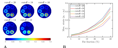
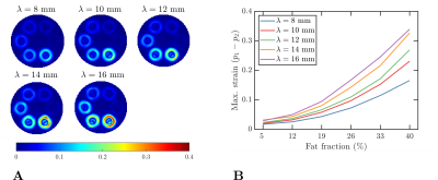
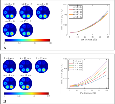
Figure 2 shows the results obtained in the first experiment. Overall, smaller strains were observed for smaller cutoff frequencies, and the biggest strain was obtained with the biggest fat fraction (as expected). Similarly, Figure 3 shows the results obtained in the second experiment, where the strain growth for larger tag periods (i.e., bigger encoding frequencies $$$k_e$$$).

Figure 4 shows the same results described in the previous paragraph but for the phantom with smooth fat fractions (see Figure 1B). For the fixed tag period and varying cutoff frequency experiment, the trend obtained with the sharp phantom was not visible, whereas for the second experiment, the same trend was observed.

Figure 5 shows the strain curves obtained from the dynamic phantoms for six different segments. In this experiment, increasing variability between segments was observed for increasing fat fractions.

Discussion and conclusions

In presence of sharp water-fat interfaces, the displacement (induced by off-resonance effects) between two adjacent pixels is given by $$$\phi_{tag}/k_e$$$, which explains why for larger tag periods (i.e., bigger encoding frequencies $$$k_e=2\pi/\lambda$$$) the estimated strain is bigger (see Figures 3 and 4B). Similarly, the strain is susceptible to the filter cutoff frequency, i.e., to the filter bandwidth. A smaller cutoff frequency implies a smaller filter bandwidth, which produces a reduced image resolution. In other words, the filter makes the sharp transition smoother and reduces the estimated strain.

However, the effect of the bandwidth of the filter was not observed in the experiment with smooth fat fractions (see Figure 4A), which is explained by the already smooth transitions between places with and without fat (see Figure 1B). In other words, the reduced filter bandwidth generates transitions that are not smoother than the transition generated by the phantom.

Finally, the variability observed in the dynamic experiment (see Figure 5) can lead to wrong conclusions about the pairment of the left-ventricular contraction.

We presented a set of experiments demonstrating that fat can bias strain estimation from tagged MR images. The following steps are (1) to include artifacts generated during the readout to estimate and separate its effect from the preparation and (2) to perform the same experiments with in-vivo data.

Acknowledgements

The authors thankfully acknowledge the financial support of the 2021 Postdoctoral Fellowship of the School of Engineering at Pontificia Universidad Católica de Chile, the project ANID-FONDECYT 1181057, and the ANID - Millennium Science Initiative Program - NCN17\_129.