4404
Optimization of Arterial Input Function Selection for Quantitative Head and Neck Dynamic Contrast-Enhanced (DCE) MRI1Radiology and Imaging Sciences, University of Utah, Salt Lake City, UT, United States, 2Biomedical Engineering, University of Maryland, Baltimore, MD, United States, 3Radiation Oncology, Huntsman Cancer Institute, Salt Lake City, UT, United States
Synopsis
Arterial input functions measured in T1 weighted low tip angle SPGRE DCE MRI acquisitions may violate an important assumption used when modeling the conversion of image values to quantitative results: that all tissues of interest have reached steady state within the imaging volume. For arterial flow along the short axis of the imaging volume, blood may not dwell within the imaging volume long enough to reach steady state. We study both the location from which AIF will be measured and the acquisition parameters employed in order to optimize the accuracy of the DCE derived quantitative results.
Introduction
In DCE-MRI, images are acquired repeatedly over time to record contrast agent uptake by tissues of interest. The temporal image signal is converted to contrast concentration (Table 1) and used with physical models1,2 to derive quantitative measures of tissue perfusion and permeability. In head and neck DCE where arterial flow velocities are high, care must be taken when selecting the image-based arterial input function (AIF)3-5 used in the DCE models. The effect of the selection of AIF on quantitative DCE parameters has not been fully investigated. The purpose of this study is to evaluate the effect of AIF sampling location along the cranial-caudal direction on the AIF itself and the impact of AIF sampling location on the quantitative values of DCE metrics in head and neck cancer (HNC) patients.Methods
DCE Model Dependence On AIF LocationThis study is part of the prospective single arm cohort study of newly diagnosed HNC patients. The study was approved by the institutional IRB, and all patients provided written informed consent. We acquired axial DCE data volumes centered on the primary tumor (see Table 2). The AIF was measured at each slice location for either the common (CCA) or the internal carotid arteries (ICA). A 15x15 voxel region of interest (ROI) of muscle was manually selected in the posterior paraspinal muscles on the axial images. An independent variable flip angle (VFA) T1 mapping (see Table 2) was acquired to estimate the T1 in muscle. DCE analysis was performed with code written in Python implementing the extended Tofts Model4 and assuming native T1 for blood = 1650ms.
Modeling Steady-state in Arterial Signal
We modeled the blood signal (T1[C]=0=1650ms) using Equations 1-3 (Table 1) for a range of contrast concentrations, [C], repetition times, TR, flip angles, $$$\alpha$$$, and r1=4.3 (L/mmol-s). We define convergence for Equation 2 (Table 1) as approaching 90% of the equilibrium value given by Equation 3 (Table 1). Assuming the arterial spins flow with a mean velocity of 100mm/s, we compute the distance traveled before reaching convergence.
Results
Figure 1 shows examples of AIF obtained at different locations along the Z-axis (cranial-caudal direction). AIF curves obtained at the entry-level (inferior along the Z-axis – darker blue) reflect inflow effects, showing little change over time despite passage of the contrast bolus. The AIF temporal shape evolves as a function of position along the Z-axis until it resembles a more typical AIF. At the more superior slices (red), the AIF shape begins to degrade, possibly due to a non-ideal profile from the slab selective RF pulse and/or the decreasing signal intensities as the flowing spins approach steady state.Figure 2 shows the computed kTrans for muscle as a function of the slice location of the AIF sampling. Where the AIF converges in shape in the 3rd axial quarter of the volume, the kTrans converges to previously reported values for muscle kTrans 6, 0.3-0.5 per minute. The variation in kTrans across muscle ROI also reaches a minimum in this region, suggesting the optimal AIF location for our particular imaging protocol appears to be in 75-80% of the imaging volume location in the cranial-caudal direction.
Figure 3 (A and B) shows iso-contours of the distance traveled by flowing (100 mm/s) blood before reaching a 90% steady-state for selected flip angles and TR. Velocities in the CCA and ICA are respectively on the order of 800-1000 mm/s at systole and on the order of 200-300 mm/s at diastole7,8. It is then likely the arterial spins in our patient DCE acquisitions reached steady-state within the imaging volume for diastolic velocities but not for systolic velocities. For the acquisition parameters in Table 2, for arterial spins to approach steady-state at systolic velocities and peak contrast bolus concentration near 2 mmol/L the size of coverage along the Z-axis would need to be at least 25cm.
Discussion
Despite the potential of DCE imaging to provide perfusion and permeability information, quantitative DCE analysis presents tremendous challenges for translation to clinical practice in HNC. One challenge is related to the T1 mapping of original tissues and another is the optimization of AIF measurement. As a part of our prospective study investigating multi-parametric MRI, including DCE, we have realized that optimizing and standardizing the measurement of AIF is critical for accurate quantitative analysis of DCE data for HNC patients.Conclusion
When employing AIF measured directly from DCE-MRI images, it is crucial to consider acquisition parameters and blood velocities that determine how far blood will flow in its approach to steady-state. The acquisition parameters TR, TE and $$$\alpha$$$ should be chosen to ensure the particular tissues of interest reach steady-state during acquisition, accounting for the uptake of contrast agent. Measuring AIF toward the downstream end of the imaging volume provides a more robust AIF with lower variation in computed DCE parameters like kTrans. Conversely, measuring AIF in the entry-level slices of imaging volume will result in erroneous values with high variations.Acknowledgements
This pilot study was supported by the National Center for Advancing Translational Sciences of the NIH 1UL1TR002538.References
1 Tofts PS, Brix G, Buckley DL, Evelhoch JL, Henderson E, Knopp MV, Larsson HB, Lee TY, Mayr NA, Parker GJ, Port RE, Taylor J, Weisskoff RM. Estimating kinetic parameters from dynamic contrast-enhanced T(1)-weighted MRI of a diffusable tracer: standardized quantities and symbols. J Magn Reson Imaging. 1999;10(3):223-32.
2 Haase A, Frahm J, Matthei D, Hanicke W, Merboldt KD. FLASH Imaging: rapid NMR imaging using low flip-angle pulses. J Magn Reson. 1986;213:533-541
3 Tofts PS, Kermode AG. Measurement of the blood-brain barrier permeability and leakage space using dynamic MR imaging: 1. Fundamental concepts. Magn Reson Med; 1991; 17:357-367
4 Cheng, HL. T1 measurement of flowing blood and arterial input function determination for quantitative 3D T1-weighted DCE-MRI. J. Magn Reson Imag. 2007;25:1073-1078
5 Garpebring A, Wirestam R, Ostlund N and Karlsson M. Effects of inflow and radiofrequency spoiling on the arterial input function in dynamic contrast-enhanced MRI: A combined phantom and simulation study. Magn Reson Med. 2011; 65: 1670-1679
6 Koopman T, Martens RM, Lavini C, Yaqub M, Castelijns JA, Boellaard R, Marcus JT. Repeatability of arterial input functions and kinetic parameters in muscle obtained by dynamic contrast enhanced MR imaging of the head and neck. Magn Reson Imaging. 2020 May;68:1-8
7 Harloff A, Zech T, Wegend F, Strecker C, Weiller C, and Markl M. Comparison of Blood Flow Velocity Quantification by 4D Flow MR Imaging with Ultrasound at the Carotid Bifurcation. AJNR; 2013; 34(7):1407-1413
8 Maier IL, Hofer S, Joseph AA, Merboldt KD, Tan Z, Schregel K, Knauth M, Bahr M, Psychogios M, Liman J, Frahm J. Carotid artery flow as determined by real-time phase-contrast flow MRI and neurovascular ultrasound: A comparative study of healthy subjects. Euro J Rad. 2018; 106:38-45.
Figures
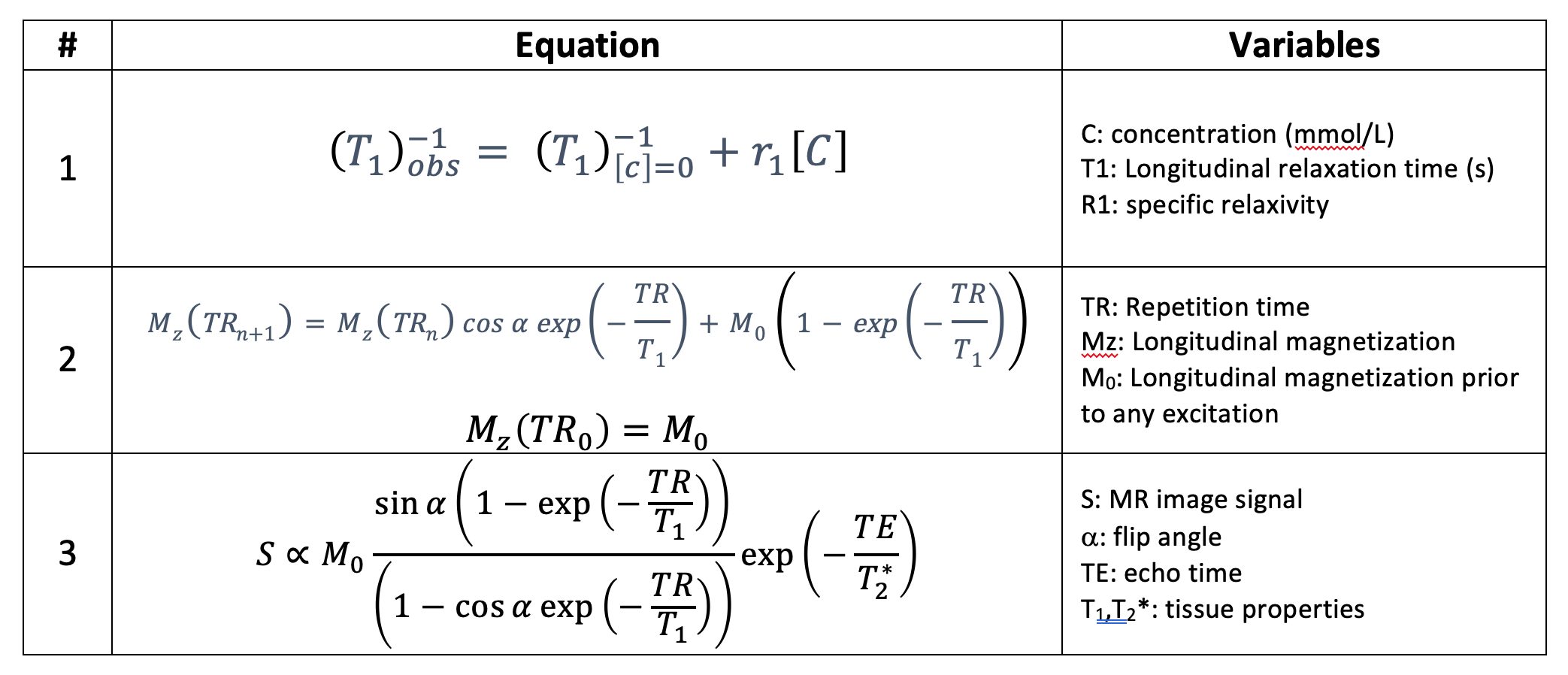
Table 1: Relevant equations and parameters used in converting DCE image intensities to concentration as well as measuring and modeling the velocity effects on AIF. With an independent measure of T1 and ignoring T2* effects, Equations 1 and 3 are combined to solve for contrast, [C]. The process first requires estimating M0 of the pre-contrast signal with known T1. Knowing M0, one then solves for the unknown T1 in the signal following contrast administration.
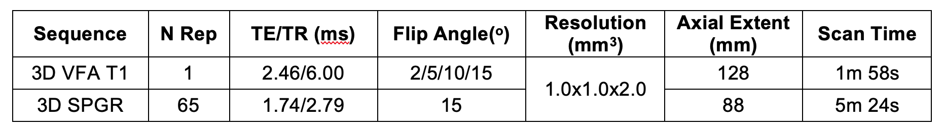
Table 2: Acquisition parameters for T1 and DCE measurements. All MRI studies were performed on a 3T scanner (Prisma, Siemens) using a 20 channel head and neck coil. The contrast administration protocol for DCE was Prohance, 0.1 mmol/kg, 5 seconds contrast bolus followed by 20 mL saline with the same injection rate.
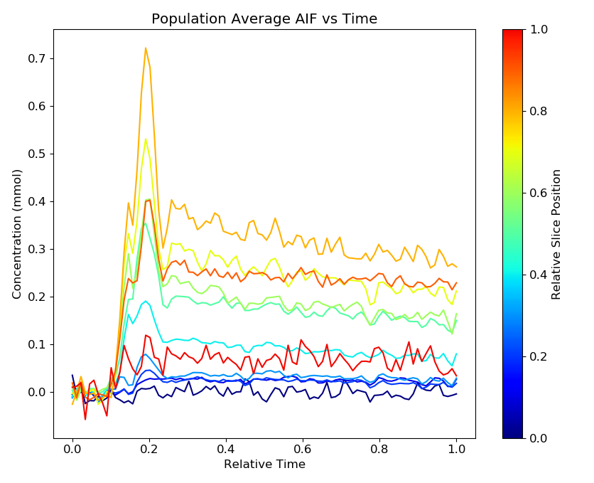
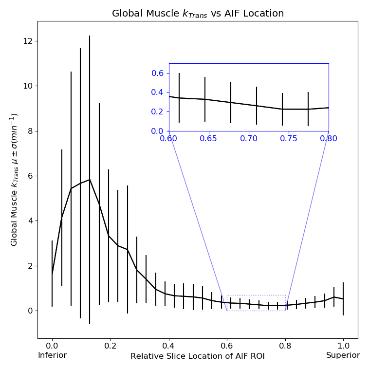
Figure 2: Computed kTrans values for posterior neck muscle averaged across 7 HNC subjects versus the relative slice position from which the model input AIF was measured. For the extended Tofts DCE model3, the muscle signals were measured in manually selected 15x15 voxel ROI positioned mid-axially for each subject. Input AIF were measured at multiple slices within the imaging volume. Error bars indicate the variation in kTrans values across the 15x15 voxel ROI. Inset shows detail for relative positions 0.6 through 0.8.
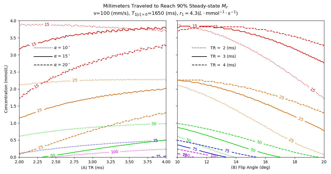
Figure 3: Distance traveled by moving (100 mm/s) blood (T1=1650ms) upon reaching 90% steady-state during a low flip angle SPGRE acquisition as a function of contrast concentration, TR and flip angle. (A) Distance contours at three flip angles as a function of concentration and TR. (B) Distance contours at three TR as a function of concentration and flip angle. At a tip angle of 15o and TR of 3ms (shown as solid contour lines in A and B), blood moving at 100 mm/s will have moved 25 mm (orange) at a concentration of 1.75 mmol/L Blood moving at 200 mm/s will move twice as far at this concentration.